RANDOM CLOSED SET MODELS: ESTIMATING AND SIMULATING BINARY IMAGES

RANDOM CLOSED SET MODELS: ESTIMATING AND SIMULATING

BINARY IMAGES

´A

M

G

A

S

´

Department of Mathematics, University Jaume I, 12071 Castell´on, Spain. e-mail: [email protected]

(Accepted November 3, 2003)

ABSTRACT

In this paper we show the use of the Boolean model and a class of RACS models that is a generalization of it to obtain simulations of random binary images able to imitate natural textures such as marble or wood. The different tasks required, parameter estimation, goodness-of-fit test and simulation, are reviewed. In addition to a brief review of the theory, simulation studies of each model are included.

Keywords: Boolean model, germ-grain model, parameter estimation, simulation.

INTRODUCTION

There are many practical situations in which the imitation of natural textures such as marble or wood is of great interest. In other words, apparently equal but random binary or gray level images must be obtained. Examples include textile and tile manufacture. Stochastic Geometry is a branch of Applied Probability that provides very powerful tools for this task. In particular, Random Closed Sets (RACS) models can be used. The most widely known and used Random Closed Set model is the Boolean model. In this paper we show how the Boolean model and a class of RACS models that is a generalization of it, can be used to obtain these simulations. With the exception of one case, we consider only binary images because the corresponding mathematical techniques are simpler and better developed. In any case, a grey level image can be transformed to a family of binary images by means of a family of thresholds.

If we want to use a RACS model to simulate similar images to a natural one these steps should be followed. A model that fits the data should first be found. Then the goodness of this fit should be checked. Thirdly the parameters of this model should be estimated from the observed image. Finally the simulation can be carried out. All these steps are considered in this paper. A brief review of the theory of the Boolean model and the most important generalizations of it is provided. These include germ-grain models, three phased models and Poisson-Boolean models. Parameter estimation methods and simulation algorithms are proposed for each of these models. In order to evaluate the goodness of the fit, the Monte Carlo test should be used and this is also briefly reviewed in this paper.

We have written a library of functions to be used with MATLAB1_{, to carry out the different tasks}

that we refer to: parameter estimation, goodness-of-fit test and simulation. This library is available at http://www3.uji.es/ simo.

There is a vast literature about Random closed Set Models, mainly about Boolean Model. But many of the papers are focused on theoretical properties and most of them are devoted to a particular model. The goal of this paper is to put together the most useful and interesting models and to emphasize their practical aspects, doing them easy to use. Although the statistical methods proposed are mainly well-known, specially those of section “The Boolean model”, as far as we know they never have been used in other kind of models like those of Section “Non-homogeneous germ-grain model” and “Three-phase Boolean model or sinter textures”.

The rest of the paper is organized as follows. The next section begins with the definition of RACS and general properties are reviewed. The second section is devoted to the Boolean model: definition, basic properties, parameter estimation and simulation. In the third section the same is carried out for the Boolean model generalizations. Finally, conclusions and future research are given in the fourth section.

RANDOM CLOSED SETS

DEFINITIONS AND ESTIMATORS

Random closed sets are mathematical models for irregular random area patterns whose formal definition

was provided by Matheron (1974). A random closed set (RACS) Ξ is a random variable taking values in

σf , the class of closed subsets in the Euclidean

space,IR2_{, with theσ-algebra generated by the Hit or}

Miss topology.

The RACS models considered here will be, with the exception of one case, stationary and ergodic. Stationarity means that its probability distribution is invariant against translations. A RACS is said to be ergodic if its mean characteristics can be obtained from spatial averages of the functional of this RACS.

The parameters of the probability distribution of a RACS can be classified into two types: aggregate and individual. The former are directly observable and can thus be easily estimated by using the ergodic property. Their definitions and estimators are common to all the RACS models. The latter are not directly observed, although they are of greatest interest when fitting a model to real data and they are specific to each model. Individual parameters have to be estimated through estimates of aggregate parameters and their estimation is very difficult except in the Boolean case. In this section the most important aggregate parameters of a general stationary RACS model are studied.

The probability distribution of any general RACS is uniquely determined by its capacity functional (Matheron, 1974);

TΞ

K P

Ξ K

/0 (1)

whereKis any compact subset ofIR2_{. IfΞis observed}

in a windowW, an unbiased estimator of T will be given by:

ˆ TΞ

K

A

Ξ K˘

W K

A

W K

where Ξ K˘ is the dilation of Ξ with K, W K the

erosion and for B IR

2_{, A}

B denotes the area ofB.

We will call ˆTΞ the empirical capacity functionalofΞ and it is a consistent estimator ofTΞ.

The simplest aggregate parameter of a RACS is the area fraction that is defined as the mean of the area of

Ξin a unitary windowW:

p E

A

Ξ W P

0 Ξ

An unbiased estimator ofpis:

ˆ p

A

Ξ W

A

W

(2)

A further, very useful aggregate functional parameter is the contact distribution function, which

provides a kind of measurement of ‘size’ when identification of single particles is inappropriate. The definition of the contact distribution function depends on the choice of a structuring element B. If B is a compact set containing the origin, then the contact distribution function is defined by:

HB

r 1

1 TΞ

rB

1 p

(3)

forr 0. The cases of particular practical importance

are the linear contact distribution function where B is a segment of unit length and the spherical contact distribution function whereB B

0

1 is a unit disk.

The contact distribution function can be estimated by combining the estimators of the capacity functional and the area fraction.

The last three reviewed aggregate parameters are less important, they are defined only for Random Closed Sets that fulfill certain conditions of regularity (convexity, smooth boundary,. . . ) and will be used only in the Boolean case.

The specific convexity number,N

A, of a stationary

and isotropic RACS is defined as the average number of exposed tangent points in a given direction. The estimation of the specific convexity number can be performed as follows. We choose an arbitrary direction u and we count the number of tangent points in the directionuinside the windowW,N

N

u W . Thus

ˆ N

A

N

N

u W

A

W

is a strong consistent estimator ofN

A.

The specific boundary length, LA of Ξ is its

expected boundary length per unit area. The following is an unbiased estimator (Weil and Weaieacker, 1984):

ˆ LA

U

Ξ W U

Ξ δ W

A

W

where δ W is the upper-right boundary of W and

U

Ξ δ W

is the length of the corresponding

intersection. Simpler estimators, as for example, the length of the boundary ofΞinside W divided by the area ofW are strong consistent but biased.

Finally, the specific connectivity number χA of a

RACS is defined as the expected connectivity number per unit area, roughly speaking the mean of the difference between the number of clumps and the number of holes per unit area. An unbiased estimator of the specific connectivity number is given by

ˆ

χA

χ

Ξ W χ

Ξ δ W

A

W

where for B IR

2_{, χ}

B denotes the connectivity

MONTE CARLO GOODNESS-OF-FIT TEST

Different procedures can be found in the literature to test whether a realization of a RACS can be assumed that follows a particular model. In Molchanov (1997) some of them are proposed for the Boolean model. If we are interested in a general method, Monte Carlo methods should be used (see Diggle, 1983).

A simple exact Monte Carlo test based on the contact distribution function can be constructed as follows.

Let us firstly assume thatHB

r is known under the

null hypothesis. Let ˆH

1

B

r be the empirical distribution function

of the observed Ξ and let ˆH

i

B

r , i 2

3

s, be

the corresponding to each of the s 1 independent

simulations of the RACS model that we are assuming under the null hypothesis, we defineuisome measure

of the discrepancy between ˆH

i

B

r andHB

r over the

whole range ofr, for example

ui

ˆ H

i

B

r HB

r

2_dr

and proceed to a test based on the rank ofu1, i.e. for

a significance level α 1

k s, the Boolean model

hypothesis is rejected ifu1rankskth largest or higher.

Another possibility is to use a graphical test. The graphical procedure consists of plotting ˆH

1

B

r,Hu

r

and Hl

r against HB

r , being Hu

r and Hl

r the

upper and lower envelopes of ˆH

i

B

r , i 2

3 s.

If ˆH

1

B

r lies close to HB

r and it is between both

envelopes, there is no evidence to reject the null hypothesis.

If the theoretical distribution function HB

r is

unknown then both, the exact test and the graphical test, can still be carried out ifHB

r is replaced by

¯ H

i

B

r

1 s 1

∑

i

j

ˆ H

j

B

r

THE BOOLEAN MODEL

DEFINITION

This section is devoted to the study of the Boolean model, the most important and relatively simple example of RACS. It is both flexible and amenable to calculations.

The formal definition of Boolean model is as follows.

Definition 1 Suppose Φλ ! x1 xn #" is a

stationary Poisson point process in IR2 _{of intensityλ.}

LetΞ1

Ξ2

be a sequence of independent identically

distributed random compact sets in IR2 _{that are}

independent of the Poisson process Φλ and satisfy

EA

Ξ0 Kˇ

%$'& ∞ for all compacts K, where Ξ0 is

a random compact set of the same distribution asΞn.

The Boolean modelΞis:

Ξ)(

i

xi& Ξi (4)

The pointsxiare calledgerms, the setsΞnare known as

grainsand the random setΞ0is said thetypical grain of the Boolean model.

The value of parameterλ is said to be theintensity of the Boolean model.

A more in-depth study of this model can be found in Stoyan et al. (1995), Molchanov (1997), Cressie (1993), Ayala (1988) and Serra (1982). Boolean model applications to real images can be found in Stoyan et al. (1995), Serra (1982), Plaza (1991), Margalef (1974) and Lyman (1972).

Individual parameters of a Boolean model are the intensity of the germ process and parameters of the distribution of the primary grain.

PROPERTIES

In the Boolean model, the expression of the aggregate parameters defined in the previous section are known and relatively simple. They are reviewed in this section, and a theoretical study on them can be found in Stoyanet al.(1995) and Molchanov (1997).

The expression of the capacity functional for a Boolean model is:

TΞ

K 1

exp λEA

Ξ0 Kˇ *"+

If the primary grains are convex, the generalized Steiner formula gives for convexK:

TΞ

K 1

exp λ

¯ A&

1 2πU

K

¯ U& A

K,*"

where ¯U is the mean of the perimeter of Ξ0 and ¯A

is the mean of its area. If we substitute K for the origin, we obtain the expression of the area fraction: p 1

exp

λA¯ .

Taking into account Eq. 3, the contact distribution function of a Boolean model has the following expression

HB

r 1

exp λE-A

Ξ0 rB˘ /.

A¯

Finally can easily be shown that

N

A λ

1 p

LA λ

1 p

¯ U

and ifΞ0is convex and isotropic:

χA

1 p

λ

λ2

4π2U¯2

PARAMETER ESTIMATION

In this section we provide a brief review of methods for the estimation of numerical individual parameters of the Boolean model. As mentioned above, they are the intensity and the parameters of the probability distribution of the primary grain. A great number of methods are available which can be classified into two general types: Minimum Contrast Methods and Moment Methods. In practice we will need to combine some of them to obtain the estimation of all the parameters of the model.

Minimum Contrast Method

This method was first introduced for contact distribution functions (Dupac, 1980; Diggle, 1981) although it can be used for other aggregate functions.

Let B be a structuring element; we consider the contact distribution function HB

r (Eq. 5).

Its corresponding logarithmic transform (henceforth referred to as the logarithmic contact distribution function) is equal to:

Hl B

r log

1 HB

r

λE-A

Ξ0 rB˘ 1.

A¯

and on applying the Steiner formula (Matheron, 1974):

Hl B

r λ

A

B2&

1 2πUU¯

B,

For typical structuring elements such as disks, lines or squares, Hl

B

r is a polynomial function.

The essence of the minimum contrast method lies in finding the polynomial f

r which best approximates

the empirical logarithmic contact distribution function. The estimators of individual parameters can be obtained from their coefficients.

As an example, we can examine the case of the spherical contact distribution function. If the structuring elementBis the unit disk,

Hl B

r λπr

2

& λr

¯ U

and

Hl B

r

r λπr& λ

¯ U

is linear, if f

r a& bris fitted to it then:

ˆ

λ

ˆ b π

ˆ¯ U aˆπ

bˆ

METHOD OF MOMENTS

This method is similar to the method of moments in classical statistics, namely, the estimators of parameters for the Boolean model are chosen to match the empirical values of aggregate parameters. Individual parameters are estimated with the relations given in the previous section being taking into account:

ˆ p 1

exp λˆAˆ¯

(6) ˆ

LA

ˆ

λ

1 pˆ

ˆ¯ U

(7)

ˆ

χA

1 pˆ

ˆ

λ

ˆ

λ2

4πUˆ¯2

(8) ˆ

N

A

ˆ

λ

1 pˆ

(9)

It is worthwhile to note that the determination of ˆχA and ˆNA may be difficult in a discrete context.

With respect to the first one, it is usual that popular software package of mathematical computations, like MATLAB, has implemented efficient functions to calculate it. With respect to the second one, our experience in the practical image analysis, tell us that good results are obtained by considering as a lower tangent point, any configuration belonging to the one of the types shown in Fig. 7.

BOOLEAN MODEL SIMULATION

The simulation of a Boolean model is very simple. LetW be a rectangular window of size m3 n, λ the

germ intensity andΞ0the typical grain. The algorithm is:

Algorithm 1 1. Generate k Po

λA

W .

2. For i 1to k:

(a) Generate x

i

1 Un

0

n , x

i

2 Un

0

m , xi

x

i

1

x

i

2

(b) Generate Ξi following the distribution of Ξ0.

Po and Un denote the Poisson and the uniform

distribution respectively. In the case when λA

W is

large then some form of rejection technique must be used in step 1 (Ripley, 1987). In order to correct the edge effect, this algorithm should be applied to a larger window W4 such that the probability of a

grain centered in the boundary of W4 intersectsW is

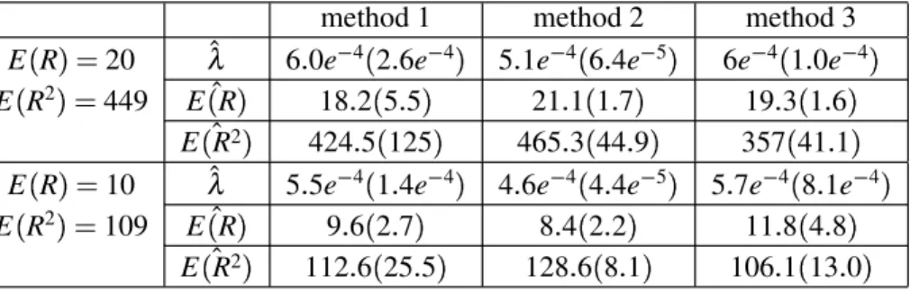
depreciable. In Fig. 1 we can see various simulations of a Boolean model in a 5123 512 window. The primary

grains are random balls, random line segments and random squares respectively.

(a) (b) (c)

Fig. 1. Three simulations of a Boolean model in a 512 3 512 window. (a) Balls with random radii

R N

10

2 andλ 0001. (b) Line segments with

random length L N

30

10 and λ 0005. (c)

Squares with random side l N

30

10 .

SIMULATION STUDY

In this section we carry out a simulation study in order to compare the performance of the different parameter estimation procedures. We simulated 50 Boolean models in a 5123 512 window whose primary

grains are random discs with Gaussian radii. Thus the parameters to be estimated are the intensity and the first and second moment (E

R ,E

R2

) of the random

radius. (We have to note that in all our simulation studies we will use E

R2

instead of the variance

because most estimation methods provide the direct estimation of this parameter). Two different intensity values were used for each experiment: 0001 and

00005. For each intensity value, two values for first

and second moments were used: (20, 449) and (10, 109).

As explained in section “Parameter estimation” a great number of methods could be used by combining the different types previously explained. We used the three following methods:

1. The first method is based on the minimum contrast method to estimate the intensity and the mean of the radius and Eq. 6 to estimate the second moment of the radius. The minimum contrast method is applied to the contact distribution function with a square as structuring element (we used a square instead of a disk because its evaluation is better in a discrete screen). We call this method 1.

2. The second method is the method of moments using Eqs. 6, 8 and 9 (in tables, method 2). 3. The last method is identical to the second one but

we use Eqs. 6, 7 and 8 (method 3).

Table 1.Results of the experimental study of Section 3.6: sample means (standard deviation) of the estimates of the different parameters for each one of the methods for a Boolean model withλ 0001.

method 1 method 2 method 3

E

R 20

ˆ

λ 12e

5

3

67e

5

4

91e

5

4

12e

5

4

15e

5

3

25e

5 4 E R2 449 ˆ E

R 261

304 238

19 173

23

ˆ E

R2

5986

6723 5297

598 325

513

E

R 10 λ 11e

5

3

18e

5

4

90e

5

4

63e

5

5

12e

5

3

99e

5 5 E R2 109 ˆ E

R 99

24 105

09 112

016

ˆ E

R2

1141

235 1339

63 1000

155

Table 2.Results of the experimental study of Section 3.6: sample means (standard deviation) of the estimates of the different parameters for each one of the methods for a Boolean model withλ 00005.

method 1 method 2 method 3

E

R 20

ˆ

λ 60e

5

4

26e

5

4

51e

5

4

64e

5

5

6e

5

4

10e

5 4 E R2 449 ˆ E

R 182

55 211

17 193

16

ˆ E

R2

4245

125 4653

449 357

411

E

R 10

ˆ

λ 55e

5

4

14e

5

4

46e

5

4

44e

5

5

57e

5

4

81e

5 4 E R2 109 ˆ E

R 96

27 84

22 118

48

ˆ E

R2

1126

255 1286

81 1061

The results are shown in Tables 1 and 2. These tables show the sample means and standard errors of the estimates of the different parameters for each one of the previous methods. It can be seen that all of them provide good estimations: The sample mean is in all cases very close to the real value and the variance is not too big except in method 1, this method is less efficient.

BOOLEAN MODEL

GENERALIZATIONS

In this section, we study some generalizations or modifications of the Boolean model that may be used for the simulation of structures of greater complexity.

GERM-GRAIN MODELS

The Boolean model presupposes very strong assumptions: homogeneous Poisson process of germs and independence between germs and grains. Unfortunately, a great number of real images cannot assume these premises. The first type of generalization of a Boolean model studied in this paper attempts to relax some of these assumptions. The relaxation of these assumptions leads to the class of germ-grain models, a general definition of which can be found in Stoyanet al.(1995) and is as follows:

Definition 2 SupposeΦλ 6 x1

xn

7" is a point

process in IR2_{. LetΞ1}

Ξ2

be a sequence of random

compact sets in IR2_{. A germ-grain modelΞis:}

Ξ (

i:xi8 Φλ

xi& Ξi (10)

The pointsxi are called thegermsand the setsΞnare

known as thegrainsof the model.

In this section we will study three particular cases of germ-grain models: cluster germ-grain model, non-homogeneous germ-grain model and Gibbs process of non-intersecting grains.

CLUSTER GERM-GRAIN MODEL

This model is defined as a germ-grain model (10) whose germ process is a cluster Poisson point process independent of the grains, and the grains are independent and identically distributed asΞ0. Note that this definition is fairly different from the definition of Boolean cluster model given in Saxl and Rataj (1996) and Rataj and Saxl (1997).

A cluster point process (Neyman, 1939; Neyman and Scott, 1979; Diggle, 1983) is generated as

follows: first, a Poisson point process of intensity ρ

is generated. This will be called the parent process. A random non negative integer is associated to each parent, the number of offsprings. The offspring of a given parent is located around its parent independently and according with a given probability distribution. The final point process is composed only of the different offspring, i.e., the parent process is not considered.

Some formulas for Cluster germ-grain models can be found in Last and Holtmann (1999).

Simulation

In order to simulate the cluster germ-grain model we simply have to substitute the germ process generation step in the Boolean model simulation algorithm 1 by:

1. Generatek Po

ρA

W

2. Fori 1 tok:

(a) Generatey

i

1 Un

0

n ,y

i

2 Un

0

m ,yi

y

i

1

y

i

2

(b) Generate li following a univariate discrete

distribution f

l

(c) For j 1 to li. Generate xi j uj & yi with

ujfollowing a bivariate continuous distribution

h

u

(a) (b) (c)

Fig. 2. Three simulations of a cluster germ-grain model in a 5123 512 window with ρ

00001, the

position of the offsprings with respect to their parents are uniform in the ball of radius40 and the number of offsprings per parent follows a discrete uniform distribution on 0

10" . (a) balls with random

radii R N

10

4 , (b) line segments with random

length L N

10

4 and (c) squares with random side

l N

10

4.

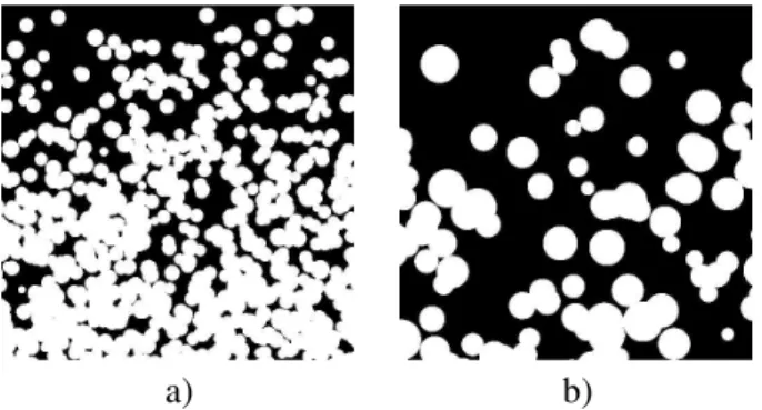
Fig. 2 shows three simulations of this model where parents have intensityρ 00001, the positions

uniform distribution on 0 10" . In the first image,

the grains are balls with random radii following a Gaussian distribution with mean, E

R9 10, and

second moment, E

R2

: 104. In the second image

they are random line segments of random length with the same distribution. The last image shows the realization of a model whose grains are random squares, again with the same distribution for their sides.

NON-HOMOGENEOUS GERM-GRAIN MODEL

A non-homogeneous grain model is a germ-grain model (Eq. 10) whose germ process is a non-homogeneous Poisson point process independent of the grains and the grains are independent and identically distributed asΞ0.

A non-homogeneous Poisson process is obtained when the constant intensity of the Poisson process is substituted by a general intensity measureΛ

A , for

A IR

2_{, usuallyΛ}

A;=< Aλ

x dx.

It can easily be shown that the capacity functional of this germ-grain model is given by:

TX

K 1

exp># E @?

˘

Ξ0 K˘ ?λ"BA

(11) with

?

˘

Ξ0 K ?λ

C

IR2IΞ˘0D K

x λ

x dx

It should be noted that this model is not stationary.

Example

Let us considerλ

x1

x2E λ0x1, i.e. the intensity

at point x is proportional to its abscisa, and Ξ0

B

0

R with randomR. A similar type of heterogeneity

is considered in Hahn et al. (1999). This model is not stationary and the definitions of the area fraction and the contact distribution function will depend on x

x1

x2 .

If we considerK B

x

t the exponent in Eq. (11)

has the expression

E

˘

Ξ0D K

λ

y dy E

F

B

xGR

t

λ0y1dyH

E >λ0x1

R& t

2_π

AI

Fort 0 the expression of the area fraction is:

p

x 1 exp

E-λ0R

2_x1π

.J

(12) and the contact distribution function is:

HB

xG1

tK 1 exp

λ0x1πt

t& 2E

R (13)

Parameter estimation

In this section we study parameter estimation in the particular non-homogeneous germ-grain model given in the example of the last section.

The capacity functional TΞ

K and the area

fraction of this model, and in general of any non stationary model, can be estimated by using a kernel estimator. Let us consider y

1 y m

" a grid of

points in the observation windowW, then we estimate the capacity functional atK B

x

t by:

ˆ TΞ B x t

∑yL

iM 8 ΞD B

0Gt k

x y

i ∑m i 1k

x y

i (14) withk

denoting a kernel function.

Note that if t 0, we have the estimation of

the area fraction. But for the type of heterogeneity considered in this example (vertical linear trend), one may estimate the capacity functional by the length fraction ofΞ K˘ along the horizontal line with abcisa

x1. Hence no bivariate kernel is needed.

Taking into account Eq. (13), we can estimate individual parameters of this model using a minimum contrast method. If we assume that radii are Gaussian, we have to estimate λ0, E

R and E

R2

. The

expression of the logarithmic contact distribution function is:

log 1 HB

xG1

t*"

t λ0x1π

t& 2E

R

Given x we can estimate λ0 and E

R by fitting

a linear function to the empirical logarithmic contact distribution function. However, a better estimation will be obtained by taking a set of points x

1 x n " ,

estimating fi

t%

log 1 HB

xG1

t*" tx

i

1 , taking

their sample mean, ¯f

t and fitting a linear function

to ¯f

t.E

R2

can be estimated from the expression of

the area fraction (12).

Simulation

The simulation of this model in a rectangular window W is again very simple. The germ process step generation in the Boolean model algorithm 1 is substituted by (see Diggle, 1983):

1. λ0 maxx 8 Wλ

x . Generatek Po

λ0

2. Fori 1 tok:

(a) generate x

i

1 Un

0

n , x

i

2 Un

0

m , xi

(b) generatep Un

0

1

– ifp $ λ

xi

λ0, generateΞifollowing the

distribution ofΞ0and drawΞi& xi

– elsexiis deleted

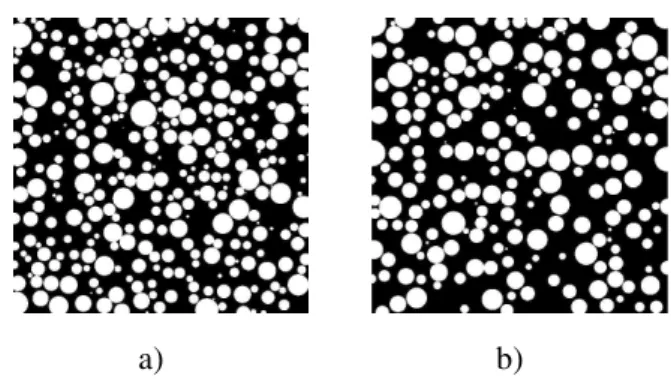
Fig. 3 shows some simulations of the example of the non-homogeneous germ-grain model given in this section with Gaussian radii.

a) b)

Fig. 3. Two simulations of a non-homogeneous germ-grain model whose intensity is proportional to the abcisa coordinate. Grains are random balls with Gaussian radii and parameters: a) λ0 000001,

E

RN 10 and E

R2

O 104, b) λ0 0000001,

E

R 20and E

R2

425.

Simulation study

A simulation study was again carried out in this section. 50 realizations of the example of the previously studied non-homogeneous germ-grain model were generated in a 512 3 512 window. The

grains are random balls with Gaussian radii and all of them have parameters λ0 2e

5

6_{, E}

RP 20

and E

R2

% 449. We estimated the parameters by

using the method explained in Section “Parameter estimation”. The results are shown in Table 3 and, as can be seen, they were quite acceptable.

ˆ

λ Eˆ

R

ˆ E

R2

3e5

6

103e

5

6

143

74 3445

1341

Table 3. Results of the experimental study of Section 4.3.4: sample mean (standard deviance) of the estimates of50realizations withλ0 2e

5

6_{, E}

RE 20

and E

R2

449.

Gibbs process of non-intersecting grains This model relaxes the assumption of independence between germs and grains in such a way that the grains do not overlap. Their formal definition is as follows (see Stoyanet al., 1995).

Definition 3 Let Ω IR

2Q

IK R w

z

K : z

IR2_;K

IK

"

LetΛ0S wn" nT 1be a point process inΩwhere:

1. zn" nT 1is a stationary point process in IR

2_.

2. Kn" nT 1i.i.d K0.

3. zn" nT 1and Kn" nT 1are independent.

Let us consider the following neighborhood relation: w1 w2iffΞ1 Ξ2

/0whereΞn Kn& zn.

Let Λ U wn" be a Gibbs process with density with

respect toΛ0:

p

w1

wn

1 z

∏

exp α& θ

wi

wj*"

where

θ

wi

wjKW

∞ if w1 w2

0 otherwise

The Gibbs process of non-intersecting grains is:

Ξ (

wn8 Λ

Ξn

This model was studied in Mase (1986) and Stoyan (1989) with circular grains. In Ayala and Sim´o (1995) this model with elliptical grains was used to model nerve fiber.

Parameter estimation

Individual parameters of this model areα and the parameters of the probability distribution ofK0. Their

estimation was studied for the case of circular grains with random radii in Stoyan (1989) and is as follows.

Let λ be the intensity of the Gibbs process,m

r

the density function of the probability distribution of the radii of the Gibbs process while p

r denotes the

probability that a disk centered in the origin and radius r intersects the Gibbs process. All these parameters are directly estimable from the observation window. Let m0

r be the density function of the probability

distribution of the radius ofK0. We have the following

relation:

λm

r e

5

α_p

r m0

r*

And the estimation ofm0

r is obtained:

ˆ m0

r

ˆ

λmˆ

r e

ˆ

α

ˆ p

r

with ˆα chosen so that:

∞

0 mˆ0

r dr 1

Simulation

Different methods of simulating general Gibbs processes can be found in the literature (Ripley, 1981; Van Lieshout, 2000), most of which are based on the so-called spatial birth-and-death (b-and-d) processes. The simulation begins with a start configuration which is then changed step by step, where points disappear (‘die’) and new ones are generated (‘born’). In our experiments, we have used a Metropolis-Hasting (M-H) type algorithm. A M-H algorithm is a discrete time Markov process where the transitions are defined in two steps, a proposal for a new state (in our case a birth or a death) is made that it is subsequently accepted or rejected based on the likelihood ratio of the new state compared to the old one. The spatial b-and-d process is a time continuous Markov process in which all transitions are accepted with probability one, but, the process stay in state x for an exponentially distributed random sojourn time. We have used one of the simplest M-H algorithm: births and deaths are equally likely and sampled uniformly.

Let W be the window where the process is generated.

Algorithm 2 1. An initial configuration Ξ0 with k

non intersecting disks is generated, with k being arbitrary. Make n k,Ξ Ξ0.

2. with probability 1 2:

(a) Generate a new point xX uniform in W and

radius rX from m0

r . IfΞ B

xX

lX

/0the new

disk is rejected. If not, i. If n Y e5

α_A

W

1 the new disk is

accepted. ii. If n e5

α_A

W the new disk is accepted

with probability eZ α_A

W

n

1 .

(b) Choose

x

r at random ofΞ.

i. If n e5

α_A

W this disk dies.

ii. If n Y e5

α_A

W

1 the disk dies with

probability n eZ

α_A

W .

Although we have choose this algorithm because it is simpler to implement, we have to warn that, in general, this algorithm could result in a low acceptance probability, especially for models exhibiting strong interaction, that would make it inefficient. In this case we should use other kind of proposals or well a spatial b-and-d process. See Clifford and Nicholls (1994) for an excellent comparison.

Another problem here is to asses how long the chain should run in order to achieve the desired

approximation. This problem could be solved by using the recently developed perfect or exact simulation (Propp and Wilson, 1996). Fig. 4 shows some simulations of this model.

a) b)

Fig. 4. Two simulations of a Gibbs process of non-intersecting grains with: a) α 3 and b) α 4,

the grains are random balls with radii following a Gaussian distribution N

20

36 .

Simulation study

In this section, a simulation study is again carried out to experimentally test the performance of the previously described parameter estimation procedure. In order to do this, we simulated 20 Gibbs processes of non-intersecting grains withα 3 and 20 withα 4.

The grains are in both cases random balls following a Gaussian distribution with first and second moment 20 and 449 respectively. The sample means and standard deviation of the estimates are shown in Table 4. The results are in general fairly good. The results forα 4

are a slightly better, they are less variable and their mean is nearer to the real value.

ˆ

α Eˆ

R

ˆ E

R2

α 3 27 (17) 235 (29) 5725 (464)

α 4 44 (067) 229 (36) 55741 (382)

Table 4. Results of the experimental study of Section 4.3.8: sample means (standard deviation) of the estimates of20realizations with E

RK 20, E

R2

449andα 3andα 4, respectively.

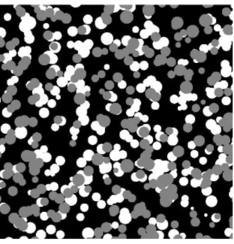
THREE-PHASE BOOLEAN MODEL OR SINTER TEXTURES

The departure from the Boolean model studied in this section consists of considering a three-phased Boolean model. This model is defined in a very simple way. Suppose thatX1andX2are independent Boolean

models. Then we define:

Ξ1 X1

Ξ2 X2 X

c

1

Ξ3 X

c

2 X1c

and we call

Ξ1

Ξ2

Ξ3 the three-phased Boolean

model. Note that the complete Boolean model X1

forms component 1. Component 2 can be interpreted as a pattern destroyed in part by X1 and Ξ3 is the

background. This three-phased model was introduced in Serra (1982) and applied to the description of sinter materials.

It can easily be shown that the area fraction fulfills:

pX2

pΞ2

1 pX

1

Parameter estimation

Since X1 is a completely observable Boolean

model its individual parameters can be estimated using the methods from section “The Boolean Model”.

In order to estimate the parameters ofX2, we can

use the equation of the capacity functional for union-censoring given in Molchanov (1997):

TX2

K

TX1[ X2

K TX

1

K

1 TX

1

K

(15)

Using Eq. (15) the contact distribution function of X2 can be estimated and the parameter of X2 can be

estimated using the minimum contrast method applied to the empirical logarithmic contact distribution function as explained in Section “The Boolean model”.

Simulation

The simulation of this model is trivial when its definition and the algorithm 1 are taken into account. Fig. 5 shows a simulation of a three-phased Boolean model, both Boolean models have intensity λ

00005 and random balls with Gaussian radii with

parametersE

R 20 andE

R2

K 449.

Fig. 5.A simulation of a three-phased Boolean model. Both Boolean models have intensityλ 00005 and

random balls with Gaussian radii with parameters E

R 20and E

R2

449.

SIMULATION STUDY

In this section we study the performance of the parameter estimation procedure, again by means of a simulation study. We applied the previously explained procedure to 20 simulations of a three-phased Boolean model. X1 and X2 are both Boolean models with

intensityλ 00005 and random balls with Gaussian

radii with parametersE

R\ 20 andE

R2

\ 449. The

results are provided in Table 5. As was expected, the estimates ofX1 parameters are more precise because

the model is completely observed.

THE BOOLE-POISSON MODEL

The last Boolean model generalization studied in this paper is obtained by restricting the Boolean realizations to remain inside the polygons generated by a Poisson process of lines. It is called the Boole-Poisson model (Serra, 1982).

Table 5. Results of the experimental study of Section 4.5: sample means (standard deviation) of the estimates of 20realizations with E

R 20, E

R2

449andλ 00005for both Boolean models.

ˆ

λ Eˆ

R

ˆ E

R2

Boolean 1 000056

000023 2253 (1452) 4838

3136

Boolean 2 (hidden) 000068 (00005) 2607 (255) 56814

6296

A line process is a random collection of lines in the plane which is locally-finite; i.e. only a finite number of lines hit each compact planar set. A line process can be seen as a particular case of point process on IR2_{, because we can parameterize it as:}

p

φ IR3

0

2π. IR

2_{, with pbeing the perpendicular distance}

S= p φ : 0 Y p

$ ∞ 0 Y φ

$ 2π"]

A line process is a point process on S. If K is a compact planar set andGK the set of lines hitting K,

the corresponding subset inS will be called SK. The

measure of these sets is given by the Lebesgue measure considered as subsets ofIR2_.

A Poisson line process is the line process produced by a Poisson process onS.

Let us now see the definition of Poisson-Boolean model.

Let X1 be an isotropic Poisson lines process in

IR2 _{with intensityλ. This process generates a random}

tessellation, each polygon Π of the tessellation is intersected with a realization of a Boolean modelX2

with intensityθand primary grainX0

2, in such way that

a different realization ofX2 is used for each polygon.

The union of all these portions of X2, together with

X1make up a setY that is called the Poisson-Boolean

model.

If T1, T2 andT

B denote the capacity functional

ofX1,X2andY respectively, we have:

T

B 1

exp λU

B

θE-A

X0 2 Bˇ

1."]

Applying the Steiner formula and taking the logarithm, we obtain the following expression:

log 1 T

B^"_ λU

B&

θ ` A

X0 2&

1 2πU

X0 2U

B2& A

Bba (16)

This equation together with the expression of the area fraction:

p 1

exp θA

X0 2*"

(17)

and will be used in the next section to estimate the parameters of the model.

Parameter estimation

Individual parameters of this model are the individual parameters of the Boolean model. To estimate them we previously need to estimate the intensity of the line process. This is an aggregate parameter and it can be estimated as a spatial mean.

ˆ

λ

Number of lines intersectingW A

SW

However, this estimation has added difficulties in practice. The lines in the image have to be counted automatically, which is not a simple task. To count the number of lines in the image we take into account the

fact that this number is equal to the number of local minima of the Radon transformation of the image.

Once λ has been estimated, we again use the minimum contrast method to estimate the rest of the parameters of the model. From Eqs. (16) and (17) we obtain the expression of the logarithmic spherical contact distribution function

log 1 HB

r^"

r λ8& θ 1

2πU

X0

2 8& 9rK

The estimates are obtained by fitting a linear function to the empirical function.

SIMULATION

The simulation algorithm of this model has two basic steps. In the first step the lines process is generated and in the second, a Boolean model is simulated in each polygon following algorithm 1. The simulation of the line process step is as follows (Stoyan and Stoyan, 1994):

(i) Let W be the window where the process is to be simulated (To simplify the simulation we assume that W is square). Find the set SW in S and its

Lebesgue measure. (IfW is convex, as in this case, this is the measure of the boundary ofW)

(ii) Generate a Poisson-distributed random number n with parameterλA

SW .

(iii)Generate n independent random lines using the following steps (to simplify the notation, assume thatWis the unit square):

1. u Un

0

1

2. Ifuc

1

d

2go to (5)

3. v Un

0

1

4. p

u

d

2:φ 2πv: go back to (1)

5. v Un

0

1:φ 2πv

6. T fe 2

sin

φ2& cos

φ

7. Ifuc T then (1)

8. p

u

d

2: go back to (1).

(a) (b)

Fig. 6. Two simulations of a Poisson-Boolean model where the grains are random balls with radii following a Gaussian distribution with parameters (a) λ

00001,θ 0001, E

R 20and E

R2

449; (b)

λ 00005,θ 0002, E

R 10and E

R2

109.

Fig. 7. Pixel patterns used to detect lower tangent points.

Simulation study

In this section, we again carry out a simulation study to show the performance of the former method. We simulated 20 Poisson-Boolean model realizations with parametersλ 0002,θ 000005. The grains

of the Boolean model are balls with random radii following a Gaussian distribution withE

R 20 and

E

R2

449. The results can be seen in Table 6. They

are relatively good in the estimation of λ and θ, a slightly less so for the mean of the radius and not so good for the variance.

CONCLUSIONS

In this paper we reviewed the use of Random Closed Sets as a powerful tool in simulating random binary images able to imitate natural textures. The Boolean model and a class of RACS models that is a generalization derived from it have been studied. For each model simulation algorithms and parameter estimation procedures were given.

In addition a library of functions to be used with MATLAB was written to carry out the different tasks that we refer to.

Future work could include other generalizations of Boolean Model with different point processes like Strauss point processes or area-interaction point processes.

ACKNOWLEDGMENTS

We would like to thank to the anonymous referees for correcting errors and improving the paper. This work has been partially funded by grants GV01-307 and BSA2001-0803-C02

Table 6. Results of the experimental study of Section 4.7.1: sample means (standard deviation) of the estimates of a Poisson-Boolean model withλ 0002,θ 000005, E

R 20and E

R2

449.

ˆ

λ _θˆ _Eˆ

R

ˆ E

R2

0001 (584e

5

7_{) 0}

00008 (341e

5

5_{) 15 (10}

39) 1306 (546)

REFERENCES

Ayala G (1988). Inferencia en Modelos Booleanos. Tesis Doctoral. Universidad de Valencia.

Ayala G, Sim´o A (1995). Random closed sets and nerve fiber degeneration. Adv Appl Probab 27:293–305. Clifford P, Nicholls G (1994). Comparison of

birth-and-death and metropolis-hastings markov chain monte carlo for the strauss process. Tech. rep., Manuscript. Oxford University.

Cressie N (1993). Statistics for spatial data. Wiley Series in Probability and Mathematical Statistics.

Diggle P (1981). Binary mosaics and the spatial pattern of heather. Biometrics 37:531–9.

Diggle P (1983). Statistical analysis of spatial point patterns. Academic Press.

Dupac V (1980). Parameter estimation in the poisson field of disc. Biometrika 67:187–90.

Hahn U, Micheletti A, Pohlink R, Stoyan D, Wendrock H (1999). Stereological analysis and modeling of gradient structures. J Microsc 195:113–24.

Last G, Holtmann M (1999). On the empty space function of some germ-grain models. Pattern Recognition 32:1587– 600.

Mase S (1986). On the possible form of size distributions for gibbsian processes of mutually non-intersecting balls. Appl Prob :646–59.

Matheron G (1974). Random Sets and Integral Geometry. New York: J. Wiley and Sons.

Molchanov I (1997). Statistics of the Boolean Model for Practitioners and Mathematicians. Wiley Series in Probability and Mathematical Statistics.

Neyman J (1939). On new class of contagious distributions, applicable in entomology and bacteriology. Ann Math Statist 10:35–57.

Neyman J, Scott E (1979). Statistical aproach to problems of cosmology (with discussion). R Statist Soc B 20:1–43. Plaza M (1991). Contrastes en modelos germen y grano.

Tesis Doctoral. Universidad de Valencia.

Propp J, Wilson D (1996). Exact sampling with coupled markov chains and applications to statistical mechanics. Proceedings of the Seventh International Conference on Random Structures and Algorithms 9:223–52.

Rataj J, Saxl I (1997). Boolean cluster models: mean cluster dilations and spherical contact distances. Math Bohem 122:21–36.

Ripley B (1981). Spatial Statistics. J. Wiley and Sons. Ripley B (1987). Stochastic simulation. J. Wiley and Sons. Saxl I, Rataj J (1996). Spherical contact and nearest

neighbour distances in boolean cluster fields. Acta Stereol 15:91–5.

Serra J (1982). Image analysis and mathematical morphology. Academic Press.

Stoyan D (1989). Statistical inference for a gibbs point process of mutually non-intersecting discs. Biometrik J 31:153–61.

Stoyan D, Kendall W, Mecke J (1995). Stochastic Geometry and its applications. Chichester: J. Wiley and Sons. Stoyan D, Stoyan H (1994). Fractals, random shapes and

point fields. Methods of geometrical statistics. Wiley series in probability and mathematical statistics. Van Lieshout M (2000). Markov point processes and their

applications. Imperial College Press.