Data Fusion Method Based on Adaptive Kalman Filtering

Data Fusion Method Based on Adaptive Kalman Filtering

Bernadus Herdi Sirenden

Research Center of Metrology LIPI, Puspiptek Serpong, South Tangerang 15311, Banten

e-mail: [email protected]

Abstract

This paper discusses data fusion methods to combine the data from a rotary encoder and ultrasonic sensor. Both sensors are used in a micro-flow calibration system developed by the Research Center of Metrology LIPI. The methods studied are hierarchical data fusion and Kalman filtering. Three types of Kalman filters (KFs) are compared: the conventional Kalman filter and two adaptive Kalman filters. Moreover, a method to combine the uncertainty results from KF in hierarchical data fusion is proposed. The aim of this study is to find appropriate methods of data fusion that can be implemented in micro-flow calibration systems. Data from two experiment setups are used to compare the methods. The result indicates that one of the methods (with little adjustment) is more appropriate than the other.

Abstract

Metode Penggabungan Data Berdasarkan Adaptive Kalman Filtering. Makalah ini membahas tentang metode fusi data antara rotary encoder dan sensor ultrasonik. Kedua sensor yang digunakan pada sistem aliran kalibrasi mikro yang dikembangkan oleh Pusat Penelitian Metrologi LIPI (RCM-LIPI). Metode yang dikaji dalam makalah ini adalah fusi data hierarkis dan Kalman Filter. Tiga jenis Kalman Filter dibandingkan dalam makalah ini, konvensional dan dua metode adaptif. Makalah ini juga mengusulkan metode untuk menggabungkan hasil ketidakpastian dari Kalman Filter dalam fusi data yang hiearkis. Tujuannya adalah untuk menemukan metode yang tepat, serta dapat diimplementasikan untuk sistem aliran kalibrasi mikro. Data dari dua konfigurasi percobaan digunakan untuk membandingkan metode-metode tersebut. Hasilnya mengarah ke kesimpulan bahwa salah satu metode (dengan sedikit penyesuaian), lebih tepat daripada lainnya.

Keywords: data fusion, adaptive Kalman filter, encoder, ultrasonic, micro-flow

1.

Introduction

This paper discusses methods of data fusion to combine the data from rotary encoder and ultrasonic sensor. Both sensors are used in micro-flow calibration system developed by Research Center of Metrology LIPI (RCM-LIPI). The system consists of a double (twin) metallic syringe. This double syringe is moved back and forward by a linear actuator, so the system generates constant flow rate.

The linear actuator consists of a low-speed DC motor connected to a ball screw module. The rotary encoder is attached to a motor to measure its angular speed. Previously, RCM-LIPI had tried to develop a micro-flow calibration system using a single glass syringe and used only rotary encoder as displacement and velocity sensor; the result was not satisfactory [1].

Therefore, in this development, an ultrasonic sensor is added to improve measurement result. An ultrasonic

sensor is attached to the other side of the double syringe, and it measures the position of stainless steel plane attached to the piston rod of syringe. The plane will dynamically move following the piston movement.

Federico Castanedo briefly defined data fusion as “combination of multiple sources to obtain improved information; in this context, improved information means less expensive, higher quality, or more relevant information.” He classified available data fusion techniques into three nonexclusive categories: (i) data association, (ii) state estimation, and (iii) decision fusion. The most popular technique in state estimation is Kalman filtering [2]. In this study, a Kalman filter (KF) is used to fuse the data coming from a rotary encoder and an ultrasonic sensor.

  the unscented Kalman Filter, which uses a strategy of

sampling points around the mean [2]. The system discussed in this paper is the linear movement of double piston, which is a linear system that can be handled by a KF.

There are four architectures that can be used with a KF: centralized, decentralized, distributed, and hierarchical. Hierarchical is a combination of decentralized and distributed architectures [2]. In a centralized architecture, each sensor reports only its measurement to the fusion center, while hierarchical architecture runs its own filter and reports the state and uncertainty to the fusion center. Ivan Markovic and Ivan Petrovic conducted a comparative study on both architectures; they also proposed a solution for fusion of arbitrary filters, for example KF with particle filter, and presented a solution for the case of asynchronous data arrival [3]. R. Anitha et al. compared the following fusion algorithms: state fusion algorithm, measurement fusion algorithm, and gain fusion algorithm. State fusion algorithm is similar to hierarchical architecture, while measurement fusion is similar to centralized architecture. They concluded that state fusion algorithm outperforms the other two [4]. In this paper, a hierarchical architecture is used to combine measurements from rotary encoder and ultrasonic sensor.

The heart of the KF is the Kalman gain, which weighs the information coming from observations and predictions and then determines which information will have the most effect. This gain is influenced by uncertainties from meas-urements (R) and filtering process (Q). At the beginning of the KF algorithm development, the measurement and process noise are considered constant. But later on, these noises are commonly thought to be time-varying; there-fore, the corresponding values are not constant but uncer-tain. Many studies have been conducted to develop algo-rithms that enable adaptation of Q and R. The kind of KF that uses an adaptation algorithm is called an adaptive Kalman filter (AKF) [5]-[9].

There are many adaptive Kalman filtering techniques; one of the popular techniques is the adaptive method based on innovation or residual sequences. Innovation means the difference between the predicted state and actual meas-urement [6]-[9]. Under steady state condition, the innova-tion-based algorithm can perform well, but under dynamic situations, state correction sequence is required [9]. Inno-vation and state correction can be combined with another parameter used as a scale. The scale can be applied to adapt Q or R, and the sampling period is the parameter mostly used as a scale. Various AKF techniques also in-volve the choice of designer to adapt Q and R, or adapt either and make the other fixed [5]-[9].

In this paper, a comparative study is conducted between CKF and an AKF method proposed by Adam Werries and Jhon M. Dolan (Werries-Dolan) [9] and another proposed

by Wang Shaowei and Wang Shanming (Wang-Wang) [10].

To adapt Q, Adam Werries and Jhon M. Dolan proposed an AKF method based on state correction sequence, which is considered to be more appropriate than innovation sequence, while to adapt R, they used variance of measurement and then scaled by sampling period [9]. In this paper, some modifications are made to their method, because the calculation based on the method may produce a negative value of Q. The value of Q by definition should be positive semi-definite [11].

Wang-Wang proposed a single-dimensional AKF to estimate velocity based on measurement of incremental rotary encoder. To adapt the Q value, they proposed a method based on a virtual model. The model is based on innovation velocity, scale of sampling period, and some constants coefficient. The coefficient is determined by experience or experiments. Their method considers R to be constant, providing the encoder resolution and sampling period remain unchanged [10]. In this study, the method developed by Wang-Wang is used without modification, since it is considered to be appropriate.

Here, both methods discussed above and CKF are applied to estimate the velocity from rotary encoder measurement, and the results are compared. Only CKF is used to estimate the position from ultrasonic sensor measurement.

To determine the current predicted uncertainty of position estimation, the uncertainty result from rotary encoder filtering process is combined the with previous corrected uncertainty of ultrasonic sensor filtering process, following the uncertainty combination guide suggested in ISO GUM [12].

This paper is organized as follows. Chapter 2 discusses the mathematical model of the measurements and filtering model. Chapter 3 discusses the experiment. Chapter 4 shows the simulation results, and Chapter 5 presents the conclusions.

2.

Formulation

Rotary Encoder Measurement Model. Rotary encoder output is pulses that are related to the rotational position of the DC motor. These pulses cannot directly inform us of the angle position of the motor shaft; they only inform us of the motor shaft angle of rotation. To measure the rotational speed of the motor, one can take the derivative of pulses with respect to time, which is a frequency of the pulses. Because rotary encoder only informs us of the rotational displacement and not angle position, then this sensor is appropriate to measure rotational speed.

This method calculates the rotational speed of motor based on the number of pulses in constant time slice [10], which is formulated as follows:

ω

m

where T is the sampling period (s), mk is the number of

pulses in sampling period k, l is the encoder resolution

(pulses per revolution), and

ω

motor (rot/s).

Since the motor and ball screw are connected using a coupling, the rotational movement of the DC motor is related to the linear movement of the ball screw. To obtain the information regarding linear speed, we can combine the information of rotational speed of motor with information of ball screw lead, and the formulation is as follows:

ν

=ω

l

where is the lead of ball screw (mm), and e,k is the

linear speed indicated by rotary encoder at sampling peri-od k (mm/s).

Ultrasonic Sensor Measurement Model. Basically, an ultrasonic sensor measures the distance between itself and an object. The sensor transmitter transmits mechanical waves, and the sensor receiver receives the waves reflected from the object. The distance from the sensor to the object is proportional to time of flight of the waves. For the HCSR04 ultrasonic sensor, the time of flight is measured in microsecond, and the formulation to calculate the distance in cm is given by Eq. (3) as follows [13]:

𝐶𝑢 ⋅ 10 (3) where 𝑃𝑊𝑘 is the pulse width from ultrasonic sensor

(s), 𝐶𝑢 is a constant equal to 58 s/cm, and𝑑𝑢,𝑘 is the

distance of an object from the ultrasonic sensor (mm).

Since the ultrasonic sensor is fixed in this system, the sensor is suitable for measuring the position of piston, taking the sensor fixed position as a reference.

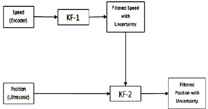
Fusion Architecture. A hierarchical architecture is used in this study. One KF will filter information coming from the rotary encoder, and the output will be the filtered value of linear speed with related uncertainty. Another KF will use that information and combine it with information from ultrasonic sensor to determine position. The architecture is described in the following Figure 1.

KF Algorithm for Rotary Encoder. The rotary encoder is only used to measure linear speed; therefore, it is independent of the ultrasonic sensor measurement.

Figure 1. Hierarchical Data Fusion

However, the ultrasonic sensor depends on the rotary encoder. The predicted position is calculated by adding the previous filtered position to the product of the filtered velocity and sampling time.

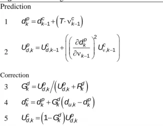
CKF Algorithm. Generally, the algorithm used for filtering measurement data from the sensor will follow discrete CKF algorithm. The algorithm is basically divided into two parts: the prediction (time update) and the correction (measurement update) as depicted in Algorithm 1.

Algorithm 1 Algorithm for Discrete KF Prediction

1 x_kpx_kc_1

2 U_kpUc_k1Q_k1 Correction

3 GkUkp





4 xc_kx_kpG z_k





5 U_kc 





where p k

x denotes predicted state at sampling period k, xp_k

denotes corrected state at sampling period k, c k

U denotes

predicted uncertainty at sampling period k, c k

U denotes

corrected uncertainty at sampling period k. Q_k denotes process uncertainty at sampling period k, G_k denotes

Kalman gain at sampling period k, R_k denotes

measure-ment uncertainty at sampling period k, and z_k denotes measurement value at sampling period k,

At the beginning of iteration (i = 1), the 𝑥0𝑐 and 𝑈0𝑐 need

  This KF is a one-dimensional filter. The filter will only

consider linear speed information. The output will be the state of linear speed and the related uncertainty. The KF algorithm is depicted in Algorithm 2 as follows:

Algorithm 2 KF Algorithm for Rotary Encoder Prediction

1   _kp c_k1

2 U_p_,k U_{ }c_{,k 1}Q_k_1

Correction

3 G_kU_p_,k













The formula to determine Q base on Wang-Wang is as follows [10]:

𝜆2𝑇2(𝜈_𝑒,𝑘𝑐 −𝜈_{𝑒,𝑘−1}𝑐 )2

1+𝛾(𝜈_𝑒,𝑘𝑐 )2

(4)

where  (s−1) and  (s2_.mm−2_{) are constant.}

The formula to determine Q base on the Werries-Dolan method, with some modification to ensure Q is a positive value, as follows:







 



, ,j ,j 1 1

1

1 N c p c c

AJ k e e k k

j

Q U U

N (5)

where N is the number of data points.

For R, the formula is

where 2 _{is the variance of measurement data or square}

of standard deviation.

KF Algorithm for Ultrasonic Sensor. Since the prediction of position is calculated based on the filtered velocity information encoder, and the uncertainty of the filtered velocity keeps updating. In this paper, that uncertainty is used as process uncertainty updating value.

The following formulation is used to filter information coming from the ultrasonic sensor. Since the hierarchical architecture is used, then the KF for ultrasonic sensor is also one-dimensional, like that of the rotary encoder. The algorithm 3 will explain in detail as follows.

Algorithm 3 KF Algorithm for Ultrasonic Sensor Prediction

1  1 





p c c

k k

k

d d T

2

2

, 1 , 1

,

1

  



_{  } 

 

  _ _{ }



 

 

p

p c k c

d k k

d k

k d

U U U

Correction

3 G_kdU_{d k}p_,





4 dckdkpG ddk









The uncertainty will be adapted from the previous uncertainty in combination with the uncertainty reported from encoder filtering process. Since the speed and position have different units, following ISO GUM [12], the uncertainty of speed is multiplied with sensitivity coefficient. Therefore, the formula of sensitivity coefficient is

𝜕𝜈_𝑘−1= 𝑇

3.

Experiment Setup

The experiment was conducted in two ways as depicted in Figure 2. First, the piston was moved from one end to another and then stopped. Second, the piston was moved forward and then backward, so that it will stop approximately at start position. Field-programmable gate array (FPGA) was used to control the piston movement based on information from encoder pulse, since the encoder is considered to be more accurate than the ultrasonic sensor.

In this study, the FPGA used was DE0-Nano from Terrasic. To control the DC motor, FPGA sends digital signal to the motor driver made by Depok Instrument. The motor itself is low rpm motor driver from Hiang Hseng. At 6 volts, the motor has 10 rpm. The motor driver linear actuator, which has 1 mm lead, was made by HIWIN [14]. The rotary encoder attached to the motor was from Autonics and has a resolution of 360 pulses per revolution [15]. The ultrasonic sensor was HCSR04, which has an accuracy of 3 mm [13]. Two pistons of 20 mL stainless steel syringe from KD Scientific were used. The rest of the mechanical system that connects all the items mentioned before was manufactured by RCM-LIPI.

The FPGA was programmed using Quartus II software from Terasic, and the programming language was the very high speed hardware description language and block diagram file (BDF). Fortunately Quartus II can obtain the data from BDF module using signal tap method; therefore, the encoder and ultrasonic sensor data can be captured. A tool command language program was made to capture the data from signal tap, create a server, and then send it to another program via TCP/IP communication. Finally, Visual Basic for Application (VBA) program was made in a macro-enabled excel file to capture and process the data from server. The sampling time used by VBA to capture data is 1 second.

To analyze the measurement result, root mean square error is used, and the mathematical equation is shown in equation (8). Wang-Wang and Werries-Dolan AKF methods are compared with the CKF result. The CKF was chosen as reference since there are no reference instrument that can be used in this experiment to validate both speed and position of piston.

𝑛∑ (𝑥𝑟𝑒𝑓𝑓− 𝑥) 2 𝑛

𝑖=1 (8)

Here, n is the number of data, and 𝑥𝑟𝑒𝑓𝑓 is reference

value

4.

Results and Discussion

Experiment 1

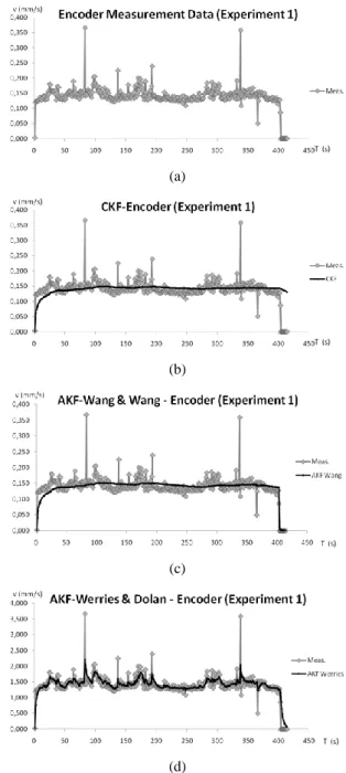
Figure 3 shows data from rotary encoder measurement for the first experiment.

Table 1 shows RMSE for Wang-Wang and Werries-Dolan methods relative to the CKF for the first experiment with encoder.

For the CKF, an initial value of R0 = 0.1 was chosen in

this study, since the distance between lead was 0.1 mm. Therefore, the uncertainty of measurement of encoder should fall between this number. For Q0 = 0.000005 and

for P0, the value was the same with R0. As we can see,

the filtering result of CKF was smooth, but it was not too sensitive to changes. As illustrated in Figure 3(b), when the speed was zero at the end of data series (the piston had stopped), CKF still indicated the piston was moving (the speed was not zero). Moreover, at the beginning of data series, the CKF result was not close to the measurement data.

(a)

(b)

(c)

(d)

Figure 3. Experiment 1 Results of (a) Encoder Measurement

Data, (b) CKF Method, (c) Wang-Wang AKF Method, (d) Modified Werries-Dolan AKF Method

Table 1. RMSEs of First Experiment with Encoder

Instrument Method

Wang-Wang Werries-Dolan

  For the AKF method proposed by Wang and Wang,  =

10 and  = 100.000 were chosen; these values are different from those Wang-Wang used in their paper [10]. The initial values of R0, Q0, and P0 were the same

with those of the CKF. As we can see, the result was as smooth as that of the CKF, and also at the beginning of the data series, the result was not close to the measurement data. At the end of data series, when the piston stopped, the result shows that the speed was zero, which is better than the CKF result.

For the AKF method proposed by Werries and Dolan subjected to a little modification, the same initial values used for the CKF was chosen. As we can see, the result had many ripples, although the ripples were not as large as those of the original measurement data. Moreover, at the first data series, the filter result was close to the measurement data. This also occurred at the end of data series, when the piston had stopped. This means this type of AKF adapts quickly to changes in situations.

From Table 1, it can be seen that the RMSEs for Wang-Wang and Werries-Dolan results relative to the CKF are almost similar, although the RMSE of the Wang-Wang is smaller.

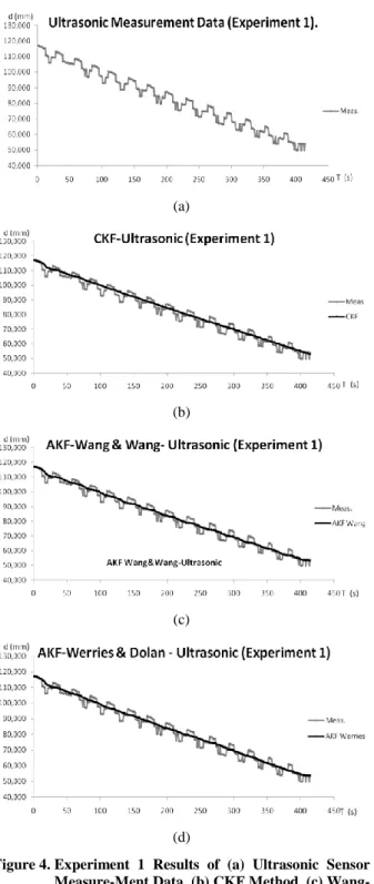
Next, we explore the results of ultrasonic sensor reading. Figure 4 shows the results of measurement data and the three different types of KF.

Table 2 shows the RMSE for Wang-Wang and Werries-Dolan methods relative to the CKF for the first experi-ment with ultrasonic sensor.

As we can see from Figure 4, the ultrasonic sensor pro-duced noisy data. The initial values of R0, Q0, P0, and X0

for all three type of KF were the same: 3, 0.000001, 3, and 117, respectively. The R0 value was derived from the

ac-curacy of HCSR04 [12], which was the same with P0. The

value of X0 was taken from a stable measurement from

ultrasonic sensor when the piston had stopped. Figure 4 also shows that the CKF and AKF proposed by Werries-Dolan presented smoother results compared to the AKF proposed by Wang-Wang. From Table 2, it can be seen that error from Wang-Wang result relative to the CKF was slightly higher than that of Werries-Dolan.

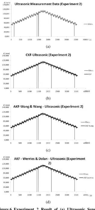
Experiment 2

The second experiment was conducted with the piston moving back and forward so that it stopped at original position. The following graphs are the results of meas-urement data and applied KF methods.

Table 3 shows the RMSEs for Wang-Wang and Werries-Dolan methods relative to the CKF for the second experi-ment with encoder.

(a)

(b)

(c)

(d)

Figure 4. Experiment 1 Results of (a) Ultrasonic Sensor Measure-Ment Data, (b) CKF Method, (c) Wang-Wang AKF Method, and (d) Modified Werries-Dolan AKF Method

Table 2. RMSEs of First Experiment with Ultrasonic Sensor

Instrument Method

Wang-Wang Werries-Dolan Ultrasonic

(a)

(b)

(c)

(d)

Figure 5. Experiment 2 Result of (a) Encoder Measurement Data, (b) CKF Method, (c) Wang-Wang AKF

Method, (d) Modified Werries-Dolan AKF Method

Table 3. RMSEs of Second Experiment with Encoder

Instrument Method

Wang-Wang Werries-Dolan

Encoder 0.0001 0.0012

As we can see from Figure 5, the speed from the second experiment was lower than the results of the first experi-ment. Although the same voltage was applied to the DC motor driver, the driver might have malfunctioned, and thus, a reduced current was supplied to the DC motor.

The CKF and AKF proposed by Wang-Wang showed the smooth results at beginning of data series, but the CKF was not as sensitive as the other two KFs when there was change of piston movement, i.e., when the piston stopped or changed direction. At first, the AKF proposed by Wer-ries-Dolan had more ripples compared to that proposed by Wang-Wang. However, after the piston changed direction, they both presented almost the same smooth result as the CKF. The ripples in the Werries-Dolan AKF result ena-bled it have a higher RMSE than the Wang-Wang AKF. The difference between the RMSEs of both methods was more than a factor of ten.

(a)

(b)

(c)

(d)

  Table 4 shows the RMSEs for Wang-Wang and

Wer-ries-Dolan methods relative to the CKF for the second experiment with ultrasonic sensor.

As in the first experiment, we can see from Figure 6 that the AKF by Wang-Wang generated more ripples com-pared with the other two. In fact, the filtering result was almost the same as the measurement data. Table 4 shows that Wang-Wang AKF method presented a higher RMSE than Werries-Dolan AKF method.

Because the speed at the second experiment was lower than that at the first, the ripple was larger. We can see from Eq. (4) that Q depended on the value of the current speed; if the speed was low, Q was large, and vice versa. The value of encoder uncertainty depended on Q. The ultrasonic sensor uncertainty value was a combination of the initial Q and the reported uncertainty from encoder; this caused ripples in filter result. This means the AKF method proposed by Wang-Wang is influenced by the value of current speed and not only by state correction.

The problem above can be solved by changing either one or the two coefficients in Eq. (4) ,  or . Here, the parameter  was changed since it is related to sampling time (the unit of  is s−1). To prove this, we chose  to be equal to 1 second−1, and the graph of Wang-Wang AKF for experiment 2 changed as follows.

We can see from Figure 7 that the encoder result was not as satisfying as before. The RMSE for encoder in Table 5 is higher than that in Table 3, although still smaller than that of Werries-Dolan AKF. However, for ultrasonic sen-sor, the result was better than before; the ripple became smaller, and the RMSE in Table 5 is smaller than that in Table 4.

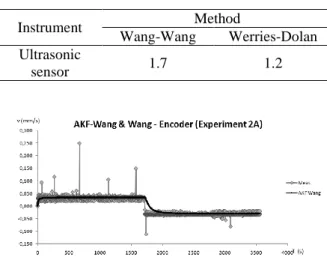
Table 4. RMSEs of Second Experiment with Ultrason-Ic sensor

Instrument Method

Wang-Wang Werries-Dolan Ultrasonic

sensor 1.7 1.2

Figure 7. Experiment 2 Result of Wang-Wang AKF Meth-od for EncMeth-oder, with Coefficient  Changed to 1 s−1

Figure 8. Experiment 2 Result of Wang-Wang AKF Meth-od for Ultrasonic Sensor, with Coefficient  Changed to 1 s−1

Table 5. RMSEs of Second Experiment for Encoder and Ultrasonic Sensor, Where  = 1 s−1

Instrument Method

Wang-Wang

Encoder 0.0003

Ultrasonic

sensor 1.1

As we can see from graphical and RMSE analyses, for rotary encoder, Wang-Wang method presented a more satisfying result compared to Werries-Dolan method. Wang-Wang AKF can filter the measurement data from the beginning of measurement, while Werries-Dolan AKF needs time for adaptation. For ultrasonic sensor result, Werries-Dolan AKF presented a more satisfying result for position determination using fusion architecture (Figure 1).

Although Wang-Wang method presented better result for encoder, it required additional appropriate tuning parame-ters, i.e.,  and . The method also depends on actual speed. Werries-Dolan method is more general, since it requires no additional tuning parameter and is independent of current speed.

5.

Conclusion and Further Work

filtered speed and position, FPGA can have a better control of piston movement.

Acknowledgements

This research is funded by RCM-LIPI trough Tematik research activity. The author would like to thanks RCM-LIPI management for the support.

References

[1] B. Sirenden, G. Zaid, P. Prajitno, Hafid, XXI IMEKO World Congress, Prague. Chez Republic., 2015, 1046.

[2] F. Castanedo, TheScientificWorldJOURNAL, Arti-cle ID 704504, http://dx.doi.org/10.1155/2013/ 704504, 2012, p.19.

[3] I. Markovic, I. Patrovic, Automatika 55 (2014) 386. [4] R. Anitha, S. Renuka, A. Abudhahir, Comput. Intell.

and Comput. Res. 2013, p.756.

[5] S.M.M, N. Naik, R.M.O. Gemson, M.R. Anantha-sayanam, Department of Electrical Engineering, Indian Institute of Technology Kanpur, India, 2015. [6] E.P. Herrera, H. Kaufmann, Proc. of the 23rd

Inter-national Technical Meeting of the Satellite Division of the Institute of Navigation, Portland, OR, USA, 2010, p.584.

[7] J.-G. Wang, S.N. Gopaul, J. Guo, CPGPS 2010 Technical Forum, 2010.

[8] P.J. Escamilla-A, N. Mort, Proc. 7th UK Workshop on Fuzzy Syst., Recent Advances and Practical Ap-plications of Fuzzy, Neuro-Fuzzy, and Genetic Al-gorithm-Based Fuzzy Systems, Sheffield, U.K., 2000, pp. 67-73.

[9] A. Werries, J.M. Auton, Vehicles, Carnegie Mellon University, US, 2016.

[10]W. Shaowei, W. Shanming, Przeglad Elektro-techniczny, 2 (2012) 5.

[11]Y. Bulut, D. Vines-Cavanaugh, D. Bernal, Proc. of the IMAC_XXVIII, Jacksonville, Florida USA, 2010.

[12]JGCM 100:2008, Evaluation of measurement data— Guide to the expression of uncertainty in measurement, 2008. http://www.iso.org/sites/JCGM/ GUM/JCGM100/C045315e-html/C045315e.html? csnumber=50461.

[13]Ultrasonic Ranging Module HC - SR04, https://cdn. sparkfun.com/datasheets/Sensors/Proximity/HCSR04. pdf.

[14]HIWIN Articulated Robot–RA605Robot datasheet, https://www.hiwin.com/pdf/ra605_robot_user_ma nual.pdf.