A common experimental design asks subjects to clas-sify a test stimulus into two categories (target or lure, Category A or B, or signal present or absent), using a binary-valued response. The resulting data can be sum-marized with two numbers: the hit rate (H), which is the probability of saying “yes” to a target, and the false alarm rate (F), which is the probability of saying “yes” to a lure. From these response proportions, one can estimate the subjects’ ability to discriminate the two classes of stimuli, as well as their general bias to prefer one response over the other. A variety of indexes meant to quantify discrimina-tion sensitivity have been proposed, including d′ (Tanner & Swets, 1954), A′ (Pollack & Norman, 1964), H 2 F, percent correct, and γ (Nelson, 1984). In this article, we examine two statistical properties of these measures that are of particular interest in an experimental setting: Type I error rate and power.
In evaluating these statistical properties, obvious con-siderations include the size of the sample and the number of trials per condition. Less obvious but equally important is the structure of evidence in the environment. We can get a sense of this structure from the receiver operating characteristic (ROC), which plots all possible (F, H) pairs as response bias varies but sensitivity remains constant. Each of the sensitivity indexes produces ROCs of a par-ticular shape, and this constrains the form of the evidence distributions that underlie the ROC (see Swets, 1986b). In other words, each sensitivity measure makes an
assump-tion about how evidence is distributed, and the degree to which the assumption matches reality will affect its statis-tical performance. As will be seen later, this factor inter-acts with the true level of sensitivity and response bias. In our evaluation, we test two types of evidence distributions most prominent in the theoretical literature: Gaussian (both equal and unequal variance) and rectangular.
Calculation of d′ as a summary of discrimination per-formance entails the assumption that the underlying dis-tributions are equal-variance Gaussian. The distance be-tween the means of the two distributions is measured by
d′ in units of their common standard deviation. It is easy to calculate:
d′5z(H) 2z(F), (1)
where the z transformation takes a response proportion and yields a z score. One advantage of d′ over other measures in this equal-variance Gaussian scenario is that it is independent of response bias. That is, the same value of d′ is observed regardless of whether subjects are relatively conservative or liberal in their “yes” responses. If the underlying distribu-tions are Gaussian but do not have a common variance, as is often the case in recognition memory tasks (Ratcliff, Sheu, & Gronlund, 1992), d′ is not independent of bias.
Calculating percent correct, p(c), as a summary statistic is appropriate when the underlying strength distributions are rectangular in form. Given equal numbers of target and lure trials at test,
389 Copyright 2008 Psychonomic Society, Inc.
Type I error rates and power analyses for
single-point sensitivity measures
Caren M. rotello
University of Massachusetts, Amherst, Massachusetts
MiChael e. J. Masson
University of Victoria, Victoria, British Columbia, Canada and
MiChael F. Verde
University of Plymouth, Plymouth, England
Experiments often produce a hit rate and a false alarm rate in each of two conditions. These response rates are summarized into a single-point sensitivity measure such as d′,and t tests are conducted to test for experimental effects. Using large-scale Monte Carlo simulations, we evaluate the Type I error rates and power that result from four commonly used single-point measures: d′, A′, percent correct, and γ. We also test a newly proposed mea-sure called γC. For all measures, we consider several ways of handling cases in which false alarm rate5 0 or hit rate5 1. The results of our simulations indicate that power is similar for these measures but that the Type I error rates are often unacceptably high. Type I errors are minimized when the selected sensitivity measure is theoreti-cally appropriate for the data.
doi: 10.3758/PP.70.2.389
sitivity statistics: (1) Given two experimental conditions that differ only in response bias, what is the Type I error rate for the (correct) null hypothesis that the mean dif-ference between the two conditions is zero, and (2) given two experimental conditions that differ only in sensitivity, what is the power of each measure to detect the sensitivity difference? The answers to these questions likely depend on a variety of factors, such as the number of subjects and trials in each condition, the magnitude of the criterion lo-cation or sensitivity differences between conditions, and the form of the underlying evidence distributions.
To our knowledge, only one study has previously asked these questions. Schooler and Shiffrin (2005) evaluated the power of d′, γ, and H 2 F to detect differences in true d′ between two conditions and the Type I error rate of each measure when the two conditions differ only in response bias. They ran Monte Carlo simulations of both experimental situations, assuming equal-variance Gauss-ian distributions. To estimate power, the simulated sen-sitivity levels were very high: d′ had an expected value of 2.5 in the weaker condition and of 3.5 in the stronger condition; the decision criterion was either unbiased, or fell one standard deviation above or below that neutral point (i.e., c 5 0, 11, or 21). The Type I error rate simu-lations used the same parameter values but made com-parisons within a particular strength condition. Their primary interest focused on cases in which a researcher is able to obtain only a small number of observations per condition per subject (i.e., 3, 10, or 20). Therefore, in addition to evaluating power and Type I error rates, using a familiar repeated measures t test, they also adopted two bootstrap-based approaches that were better suited to small sample sizes.
Schooler and Shiffrin’s (2005) findings and recom-mendations can be grouped by dependent measure (d′, γ,
H 2 F) and analysis method (t test, bootstrap methods). The corrected recognition score H 2 F performed poorly, yielding relatively low power and high Type I error rates, regardless of analysis method. Considering only the t test approach that we judge most researchers use, neither d′
nor γ was a clear winner: Although d′ had consistently higher power than did γ, that advantage was offset by a correspondingly greater Type I error rate. Given the clear desire to control Type I error rates, Schooler and Shiffrin concluded that γ is the best single-point dependent mea-sure to use with t tests.
Schooler and Shiffrin’s (2005) simulations provide some guidance for researchers conducting studies in which there are few trials per subject and high perfor-mance (d′5 2.5 or greater), as well as underlying distri-butions that are known to be equal-variance Gaussian. We were interested in exploring the properties of single-point measures of sensitivity over a broader range of experi-mental parameters. To that end, we conducted simulations that varied in the number of subjects and trials per subject, as well as the form of the underlying distributions (rect-angular or Gaussian in both equal- and unequal-variance forms). Similarly, we varied the true sensitivity levels and criterion locations over a wide range.
p( )c = 1[H + −( F)]= (H−F)+ .
2 1
1 2
1
2 (2)
As Equation 2 shows, p(c) is linearly related to the popu-lar corrected recognition score, H 2 F,that subtracts the false alarm rate from the hit rate in an attempt to correct for guessing or for response bias.
In many empirical situations, of course, the form of the underlying representation is not known. For that reason, nonparametric, “one-size-fits-all” measures of sensitiv-ity are desirable. Two putatively nonparametric measures have been proposed: A′ and γ.
A′ is an estimate of the area under the ROC. Although the area under the full ROC is a truly nonparametric measure of performance, using a single (F, H) pair to estimate that area, as in the calculation of A′, requires a number of assumptions that render A′ parametric after all (Macmillan & Creelman, 1996). A′ is consistent with rectangular distributions when sensitivity is high and with logistic distributions when sen-sitivity is low (logistic and Gaussian distributions are hard to distinguish in an experimental setting). Calculation of A′
differs for above- and below-chance performance:
`
q
A H F H F
H F H F
1 2
1
4 1
( )( )
( ) if , (3A)
and
`
q
A F H F H
F H F H .
1 2
1 4 1
( )( )
( ) if (3B)
A different apparently nonparametric measure, γ (Good-man & Kruskal, 1954), has been heavily used in the meta-cognition literature (e.g., Koriat & Bjork, 2006; Weaver & Kelemen, 1997). Nelson (1984, 1986a) argued that the sim-plest measure of a subject’s sensitivity in a task is just the probability, V, that they will judge A to have a greater value than B on a dimension of interest (say, memory strength), given that it objectively does. Nelson (1986b) showed that
γ = − = −
+ −
2 1
2
V H F
H F HF. (4)
Masson and Rotello (2007) recently showed that empiri-cally estimated γ systematically deviates from its true value unless distribution-specific correction methods are applied. Thus, γ is a parametric measure of sensitiv-ity. Masson and Rotello developed a measure called γC that assumes that the underlying strength distributions are rectangular in form and that an equal number of targets and lures are tested. In that case, they showed that
γC5 2(H2F) 2 (H 2F)2. (5) Therefore, γC is monotonic with percent correct over the range of observable (F, H) values.
Questions about the statistical properties of some of these sensitivity indices have previously been raised. The bias and precision of d′ and A′ have been studied fairly thoroughly (Hautus, 1995; Kadlec, 1999; Miller, 1996; Verde, Macmillan, & Rotello, 2006). Their robustness to violations of their equal-variance assumptions has also been explored (Balakrishnan, 1998; Donaldson, 1993; Verde et al., 2006). In this article, we ask two different statistical questions about each of these single-point
sen-rejected. A Type I error results whenever the two conditions are declared to differ reliably in terms of sensitivity. We ex-plored the performance of the various sensitivity measures in this general scenario, under different assumptions about the form of the underlying distributions and the magnitude of the response bias difference between conditions.
Calculational Methods
We ran a large number of Monte Carlo simulations under a wide-ranging set of assumptions. Figure 1 outlines the sequence of steps involved in these simulations.
Sev-Type I eRRoR RaTe SIMulaTIonS
Imagine a situation in which two conditions result in the same underlying evidence distributions but a different response bias. For example, Dougal and Rotello (2007) showed that negatively valenced emotional stimuli, relative to neutral stimuli, produce a liberal shift in response bias but leave discrimination unchanged. In experiments such as this, the researcher often conducts a t test to compare tivity in the two conditions; a correct decision for the sensi-tivity difference occurs when the null hypothesis cannot be
k
diff0
k
µ
5
d
σ
5
1/s
σ
5
1
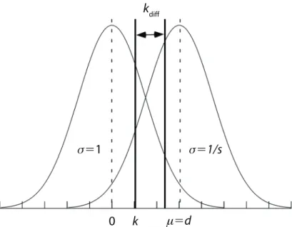
Figure 2. parameter definitions for the Gaussian distribution Type I error rate simulations.
1. Choose distributional form (Gaussian, rectangular).
Choose parameters for each of 2 conditions that differ only in: (a) criterion location ( Type I simulations)
or
(b) sensitivity (power simulations).
2. Sample T Old and T New trials in each condition for Subject i. Compute H and F rates, and apply each correction for 1 and 0. Compute all sensitivity statistics in both conditions.
3. Repeat Step 2 to generate N subjects, creating a simulated experiment. 4. Run a within-subjects t test on each dependent measure, with H0: mean
condition sensitivity difference � 0. For Type I simulations, the Null is true. For Power simulations, the Null is false.
There are 20 such t tests for each simulated experiment:
5 sensitivity statistics � 4 correction methods (none, replacement, log-linear, discard), each with a maximum of N �1 degrees of freedom.
5. Repeat Steps 2–4 1,000 times. Calculate the proportion of significant t tests for each measure � correction combination.
For Type I simulations, the proportion is the Type I error rate. For Power simulations, the proportion is Power.
6. Repeat Steps 1–5 for each combination of parameter values.
yes rate to lures in each condition divided by the number of simulated lure trials (also T). This process was repeated 10, 20, or 30 times, depending on the number of simulated subjects in each condition. Each subject in a particular simulated experiment was assumed to have the same sen-sitivity, criterion location, and criterion difference across conditions; only the sampled strengths and resulting H
and F varied across subjects.
From the values of H and F for each subject, we cal-culated five dependent measures: d′, A′, p(c), γ, and γC, as defined by Equations 1–5. One problem that research-ers face when calculating d′ is that its value is undefined whenever the hit rate is 1 or the false alarm rate is 0. A number of solutions have been proposed, including sim-ply discarding those subjects’ data. A log-linear correc-tion was advocated by Snodgrass and Corwin (1988): The number of yes responses is increased by 0.5 and the number of trials is increased by 1, so that H 5 (yes re-sponses 1 0.5)/(T 1 1) and F 5 (yes responses 1 0.5)/ (T 1 1). An advantage of the log-linear correction is that its magnitude is inversely related to sample size. Another common correction is replacement (Murdock & Ogilvie, 1968), in which a value of 0 is replaced by 0.5/T and a value of 1 is replaced by (T 2 0.5)/T. Considering only
d′, Miller (1996) found that the replacement and discard methods were equally effective at minimizing statistical bias. Kadlec (1999) noted that the log-linear and replace-ment methods performed similarly under the conditions most often observed empirically (cf. Hautus, 1995). We evaluated each of these three methods for allfive of our dependent measures. We also analyzed the results on the basis of the uncorrected measures, where possible.
One thousand simulated experiments were run for each set of parameter values; in each experiment, the subjects’ data were compared using a within-subjects t test with
α 5 .05. The number of significant t tests is the observed Type I error rate for that set of parameter values, depen-dent measure, and correction method.
Results
We present results for the dependent measures as we judge researchers to use them. Specifically, A′, p(c), and γ
are shown in their standard form, since those measures typically do not require any adjustment for values of F 5 0 or H 5 1. Indeed, that is sometimes a motivation for using such measures. We also show the Type I error rates for the new γCwithout correcting values of F 5 0 or H 5 1, so that the comparison with γ is straightforward. However,
d′ is a measure that is undefined when F 5 0 or H 5 1, and thus, correction for those values is always required. We will report the results using the log-linear correction, which typically was better than the discard method and indistinguishable from the replacement method of correc-tion in our simulacorrec-tions.
We have also chosen to summarize the data by pre-senting the results for specific parameter values that we judged to be typical of many experimental results, rather than averaging over a range of values. For all Gaussian simulations, we will report the results when there were 10 or 30 subjects in the experiments, for all four values eral parameters of our simulations reflect measures that are
under the experimenter’s control: We systematically varied the number of simulated subjects per condition (N 5 10, 20, or 30) and the number of trials per condition (T 5 16, 32, 64, or 128). In the Gaussian simulations, we assumed that the underlying evidence distributions were Gaussian in form (see Figure 2). The lure distribution was defined to have a mean of 0 and a standard deviation of 1, whereas the target distribution had a mean of d (0.5, 1, 1.5, 2, or 2.5) and a standard deviation of 1/s (see Figure 2). Because the slope of the normal-normal ROC, the zROC, equals the ratio of the standard deviations of the lure and target distri-butions, s equals the slope of the zROC. zROC slopes are typically observed to be around 1.0, with some domains consistently yielding slopes less than 1 (i.e., recognition memory; Glanzer, Kim, Hilford, & Adams, 1999; Ratcliff et al., 1992) and others yielding slopes at or above 1.0 (see Swets, 1986a, for a summary). Therefore, we set s to val-ues that span the empirically observed range (0.6, 0.8, 1, or 1.2). The criterion, k, in the more liberal condition was defined in units of standard deviation positioned relative to the mean of the lure distribution and took on values of 0, .5, and 1 (thus yielding false alarm rates of .50, .30, and .16). The criterion in the more conservative condition was shifted from k by an amount kdiff (.1, .3, .5, or .7).
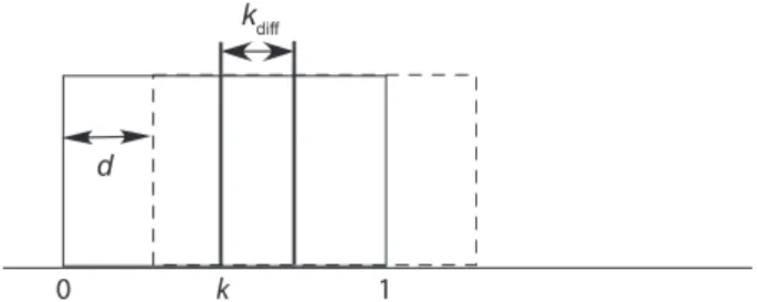
A second set of simulations assumed that the underly-ing evidence distributions were rectangular in form (see Figure 3). The lure distribution had values ranging from 0 to 1, whereas the target distribution ranged from 0 1d to 1 1d, where d equaled 0.2, 0.37, or 0.54. The criterion in the liberal condition, k, was varied over three levels (.55, .70, or .85) to yield false alarm rates of .45, .30, or .15; in the conservative condition, the criterion location was shifted by an amount kdiff (.04, .08, or .12).
For each combination of parameter values, we com-puted a hit and false alarm rate in each condition for each simulated subject. This was accomplished in several steps. First, for each subject, a set of T strength values was ran-domly sampled from each of the underlying target and lure distributions. Each of these values was compared against the criteria k and k 1 kdiff. Strengths that exceeded the relevant criterion were counted as “yes” responses to either targets or lures, depending on the distribution from which the strength had been sampled. To obtain the hit rates for that simulated subject, in each condition the yes
rate to targets was divided by the number of simulated target trials (T); similarly, the false alarm rates equaled the
d
kdiff
0 k 1
Figure 3. parameter definitions for the rectangular distribu-tion Type I error rate simuladistribu-tions.
and criterion location. Overall, the observed Type I error rates are too high to recommend γ, and no method of correcting γ for values of F 5 0 or H 5 1 alleviates the problem. Using γC (Figure 5) only exaggerates the Type I error rates, probably because this form of γC assumes that the underlying strength distributions are rectangular in form. Again, the data converge on the wrong underly-ing model, and adjustments for F 5 0 or H 5 1 do not address the problem.
The pattern of observed Type I error rates for A′ (Fig-ure 6) is less systematic than those for γ or γC, but, as for those measures, the error rates are unacceptably high under many conditions. Although the error rates in Fig-ure 6 are relatively low when slope 5 0.8, much higher error rates are observed for other values of d and/or k (see the online figures). The Type I error rates increase with subjects, trials, and the size of the difference in criterion locations. Larger values of underlying sensitivity (d) in-crease the observed error rates, and none of the methods for handling 0s and 1s help the situation.
The results for percent correct are shown in Figure 7. As for the other measures that do not assume underlying Gaussian strength distributions, the observed Type I error rate for p(c) increases with both subjects and trials as the data converge on the wrong underlying representation. The observed error rate tends to increase with the difference in criterion location, kdiff, and with the true sensitivity differ-ence, d.Adjusting the data for the presence of 0s or 1s does not reduce the error rates, which are unacceptably high. of the number of trials (16, 32, 64, 128), for two values
of the zROC slope (0.8, 1.0), for the criterion location that led to F 5 .16 in the liberal condition (k 5 1), and for criterion shifts in the conservative condition that cov-ered the range of possibilities (kdiff5 .1, .3, .5, or .7). To minimize the number of figures required, we will present only one value of true old distribution offset, d 5 1.0, but other combinations of parameter values are available online at www.people.umass.edu/caren/powerpage.html. For the rectangular simulations, we will report the results as analogously as possible. For example, we will show criterion location k 5 .85 because it leads to F 5 .15 in the liberal condition and d 5 0.37 because it yields a d′ value of approximately 0.8, values that are similar to those in the Gaussian simulations. All of the rectangular simulations had zROC slopes of 1.0.
Gaussian distributions. Figures 4–8 show the Type I error rates for γ, γC, A′, p(c), and log-linear adjusted d′, based on Gaussian distributions.
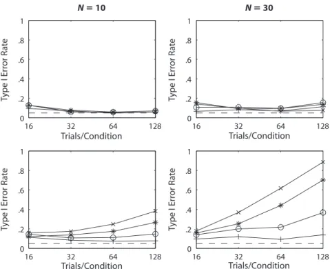
The observed Type I error rates for γ (Figure 4) were usually higher than α and increased with the number of subjects, the number of trials, and the size of the dif-ference in the criterion location, kdiff. Power is typically associated with increased sample sizes, and the effect we see here is related: Additional data provide greater convergence of the data on the underlying model, but the true model for γ is not consistent with the Gaussian model from which the data were sampled. The error rate is also affected by interactions of underlying sensitivity
16 32 64 128
0 .2 .4 .6 .8 1
N � 10
Trials/Condition
Ty
p
e
I E
rr
o
r
R
at
e
16 32 64 128
0 .2 .4 .6 .8 1
Trials/Condition
Ty
p
e
I E
rr
o
r
R
at
e
16 32 64 128
0 .2 .4 .6 .8 1
N � 30
Trials/Condition
Ty
p
e
I E
rr
o
r
R
at
e
16 32 64 128
0 .2 .4 .6 .8 1
Trials/Condition
Ty
p
e
I E
rr
o
r
R
at
e
Figure 4. Type I error rate simulations for γ, assuming Gaussian distributions, true sen-sitivity d 5 1, and k 5 1. left column, 10 simulated subjects; right column, 30 simulated subjects. upper row, zRoC slope 5 0.8; lower row, zRoC slope 5 1.0. Within each panel, the dashed line indicates α5 .05, and the solid lines reflect values of kdiff: Symbols denote
16 32 64 128 0
.2 .4 .6 .8 1
N � 10
Trials/Condition
Ty
p
e
I E
rr
o
r
R
at
e
16 32 64 128 0
.2 .4 .6 .8 1
Trials/Condition
Ty
p
e
I E
rr
o
r
R
at
e
16 32 64 128 0
.2 .4 .6 .8 1
N � 30
Trials/Condition
Ty
p
e
I E
rr
o
r
R
at
e
16 32 64 128 0
.2 .4 .6 .8 1
Trials/Condition
Ty
p
e
I E
rr
o
r
R
at
e
Figure 6. Type I error rate simulations for A′, using the same parameter values as those in Figure 4.
16 32 64 128 0
.2 .4 .6 .8 1
N � 10
Trials/Condition
Ty
p
e
I E
rr
o
r
R
at
e
16 32 64 128 0
.2 .4 .6 .8 1
Trials/Condition
Ty
p
e
I E
rr
o
r
R
at
e
16 32 64 128 0
.2 .4 .6 .8 1
N � 30
Trials/Condition
Ty
p
e
I E
rr
o
r
R
at
e
16 32 64 128 0
.2 .4 .6 .8 1
Trials/Condition
Ty
p
e
I E
rr
o
r
R
at
e
Figure 5. Type I error rate simulations for γC, using the same parameter values as those
16 32 64 128 0
.2 .4 .6 .8 1
N � 10
Trials/Condition
Ty
p
e
I E
rr
o
r
R
at
e
16 32 64 128 0
.2 .4 .6 .8 1
Trials/Condition
Ty
p
e
I E
rr
o
r
R
at
e
16 32 64 128 0
.2 .4 .6 .8 1
N � 30
Trials/Condition
Ty
p
e
I E
rr
o
r
R
at
e
16 32 64 128 0
.2 .4 .6 .8 1
Trials/Condition
Ty
p
e
I E
rr
o
r
R
at
e
Figure 8. Type I error rate simulations for log-linear d′, using the same parameter values as those in Figure 4.
16 32 64 128
0 .2 .4 .6 .8 1
N � 10
Trials/Condition
Ty
p
e
I E
rr
o
r
R
at
e
16 32 64 128
0 .2 .4 .6 .8 1
Trials/Condition
Ty
p
e
I E
rr
o
r
R
at
e
16 32 64 128
0 .2 .4 .6 .8 1
N � 30
Trials/Condition
Ty
p
e
I E
rr
o
r
R
at
e
16 32 64 128
0 .2 .4 .6 .8 1
Trials/Condition
Ty
p
e
I E
rr
o
r
R
at
e
Figure 7. Type I error rate simulations for percent correct, using the same parameter values as those in Figure 4.
Type I error rate increases with underlying sensitivity, d. It should be noted that all of the correction methods we evaluated suffer from this problem.
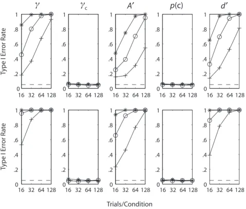
Rectangular distributions. Figure 9 shows the Type I error rates for γ, γC, A′, p(c), and log-linear d′, based on rectangular distributions. In many ways, the results of the rectangular distribution simulations are predictable from the results of the Gaussian distribution simulations: Mea-sures that assume underlying rectangular distributions perform well, and measures that assume other distribu-tional forms do not.
The error rates for γ are unacceptably high, and they tend to increase with the number of subjects and trials, as well as with the magnitude of the criterion location dif-ference, kdiff, and with true sensitivity, d (see the online figures). The reasons that γ fails here are much the same as the reasons that it fails with Gaussian underlying distri-butions: The data converge on an underlying representa-tion that differs from the model that was used to generate the data. Again, no method of adjusting values of H 5 1 or
F 5 0 reduces the Type I error rate, because the problem is structural rather than cosmetic. In contrast, the observed Type I error rates for γCare consistently low. The success of this dependent measure is due to its underlying assump-tion of rectangular strength distribuassump-tions (see Masson & Rotello, 2007).
Like γ, A′ fares poorly in these simulations. The ob-served Type I error rates are unacceptably high and tend to increase with both number of subjects and trials as the Finally, Figure 8 shows the results of using log-linear d′
as the dependent measure. This measure, unlike the oth-ers, assumes that the underlying strength distributions are Gaussian in form. Consequently, it should perform better than the other measures we have considered. However, d′
is independent of criterion location only when the under-lying strength distributions have a common variance, so we expect that log-linear d′ will perform well only when the slope of the zROC is 1.0. Figure 8 supports this con-clusion: The observed Type I error rate is near α when the slope is 1.0 and does not change with subjects or trials. However, when the zROC slope deviates from 1.0, d′ is dependent on criterion location, and therefore, the Type I error rate increases dramatically. (See Verde & Rotello, 2003, for an empirical example of how this situation can lead researchers astray.)
All is not completely well for log-linear d′, unfortu-nately, even when the slope is 1.0. As the true underlying sensitivity increases, the log-linear correction itself begins to affect the results, especially when there are small num-bers of trials per subject. This effect is caused by either the hit rate in the liberal condition reaching 1 or the false alarm rate in the conservative condition reaching 0 and being ad-justed by a relatively large amount (due to the small num-ber of trials), which reduces the estimated value of d′ in one of the two conditions. Data in the other condition are adjusted to a smaller extent, so the estimated value of d′ is more accurate. Thus, an apparent difference in sensitivity is created by the correction method; the correction-based
16 32 64 128 0
.2 .4 .6 .8 1
0 .2 .4 .6 .8 1
0 .2 .4 .6 .8 1
0 .2 .4 .6 .8 1
0 .2 .4 .6 .8 1
0 .2 .4 .6 .8 1
0 .2 .4 .6 .8 1
0 .2 .4 .6 .8 1
0 .2 .4 .6 .8 1
0 .2 .4 .6 .8 1
Typ
e I E
rr
or R
at
e
Typ
e I E
rr
or R
at
e
16 32 64 128 16 32 64 128 16 32 64 128 16 32 64 128
16 32 64 128 16 32 64 128 16 32 64 128 16 32 64 128 16 32 64 128
Trials/Condition
o
o
c A p(c) dFigure 9. Type I error rate simulations for all measures, assuming rectangular distribu-tions, d 5 0.37, and k 5 .85. upper row, 10 simulated subjects; lower row, 30 simulated sub-jects. Within each panel, the dashed line indicates α 5 .05, and the solid lines reflect values of kdiff: Symbols denote kdiff 5 .04 (plus sign), .08 (open circle), and .12 (asterisk).
Schooler and Shiffrin sampled subjects’ and conditions’ sensitivities from normal distributions and then summed. The result is that our simulations had smaller variability in
F and H across subjects and, thus, smaller standard errors for the computed dependent measures. Schooler and Shif-frin’s approach is aimed at simulating real-world variabil-ity, but it also requires making specific assumptions about the nature and magnitude of that variability. Our goal was not to estimate the Type I error rate or power in a given experiment but, instead, to provide a clean assessment of the relative performance of each of our five dependent measures across experimental situations.
Despite the differences between our approaches, we reach the same conclusions when similar parameter values are considered. For the equal-variance Gaussian distribu-tions and high true sensitivity condidistribu-tions that Schooler and Shiffrin (2005) simulated, both d′ and H 2 F yielded higher Type I error rates than did γ. Our results are con-sistent with that observation (see the online figures with Gaussian distributions, d 5 2.5, slope 5 1, k 5 0, kdiff 5 .7, trials 5 16, and N 5 30, for the closest comparison to their data) but also indicate that γ is not generally preferred over d′. For example, Figures 4 and 8 show that the Type I error rates are higher for γ than for d′ when true sensitivity is more modest (d 5 1.0).
poWeR SIMulaTIonS Calculational Methods
Our methods and assumptions for simulating power were similar to those for Type I error rate calculations. Here, however, we assumed that the two experimental conditions differed in sensitivity, but not in response bias. As for the Type I error rate simulations, we systematically varied the number of simulated subjects per condition (N 5 10, 20, or 30) and the number of trials per condition (T 5 16, 32, 64, or 128). In the Gaussian simulations, we assumed that the underlying evidence distributions were Gaussian in form (see Figure 10). The lure distribution was defined to have a mean of 0 and a standard deviation of 1, whereas the weaker target distribution had a mean of d (0.5, 1, 1.5, 2, or 2.5) and a standard deviation of 1/s, where s equaled the slope of the zROC (0.8, 1, or 1.2). The stronger target dis-tribution also had a standard deviation of 1/s, and a mean equal to d1ddiff, where ddiff 5 0.1, 0.3, . . . , 0.7, or 0.9. The criterion location, k, was defined relative to the mean of the lure distribution and took on values of 0, .5, or 1, yielding a common false alarm rate of .5, .3, or .16.
A second set of simulations assumed that the underly-ing evidence distributions were rectangular in form (see Figure 11). The lure distribution had values ranging from 0 to 1, whereas the weaker target distribution ranged from 0 1 d to 1 1 d, where d equaled 0.2, 0.37, or 0.54. The stronger target distribution was offset from the weaker dis-tribution by an amount ddiff (0.1, 0.2, or 0.3). The criterion location k was varied over three levels (.55, .70, or .85) and produced an expected false alarm rate of .45, .30, or .15, respectively.
For each combination of parameter values, we computed a hit and false alarm rate for each simulated subject, using data converge on the wrong underlying model. Although
the form of the ROC implied by A′ appears more consis-tent with rectangular distributions as sensitivity increases (Macmillan & Creelman, 1996), the Type I error rate is not consistently reduced as d increases in these simulations. As was true for γ, methods for adjusting the data for 0s and 1s do not ameliorate the problem.
Next, consider the observed Type I error rates for per-cent correct, a measure that does entail underlying distri-butions that are rectangular in form. The agreement be-tween the measure’s assumptions and the structure of the data allow percent correct to perform well: The observed error rates are consistently low.
Finally, d′ performs poorly in this simulation because it assumes that the underlying distributions are equal-variance Gaussian. The observed Type I error rates are usually very high and tend to increase with true sensitivity, more con-servative criterion location (k; see the online figures), the magnitude of the difference in criterion location between conditions (kdiff), and the numbers of subjects and trials.
Discussion
Our simulations highlight the importance of choosing a dependent measure whose assumptions correspond to the structural basis of the data. When the data come from strength distributions that are truly rectangular in form, the theoretically appropriate dependent measure,percent correct, performs extremely well, yielding appropriately low Type I error rates under a wide variety of parameter values. Similarly, the γCmeasure developed by Masson and Rotello (2007) also depends on rectangular strength distributions and performs admirably when the data are rectangular in form. All of the other dependent measures yield extremely high Type I error rates under these as-sumptions, regardless of method of adjustment for F 5 0 or H 5 1. They do so because they entail different assump-tions about the form of the strength distribuassump-tions.
When the data come from strength distributions that are equal-variance Gaussian in form, d′ is the theoreti-cally appropriate dependent measure. It performs well when sensitivity is no more than moderate; at higher lev-els of true sensitivity, the necessary correction for F 5 0 or H 5 1 tends to increase the Type I error rate. For the unequal-variance case, d′ is no longer independent of cri-terion location, and the Type I error rates are dramatically increased. None of the other dependent measures fare well when the underlying distributions are Gaussian. An obvi-ous implication of these results is that one must under-stand the data before choosing a dependent measure.
Note particularly that γ and A′, both erroneously thought to be nonparametric measures of performance (see, e.g., Macmillan & Creelman, 1996; Masson & Rotello, 2007), are poor choices for the dependent measure, regardless of the form of the underlying strength distributions: The Type I error rates that resulted for those measures were unacceptably high in both simulations.
Our simulations resulted in higher observed Type I error rates than those reported by Schooler and Shiffrin (2005). However, our simulations assumed that all the subjects had the same underlying sensitivity in each condition, whereas
their standard form, since those measures typically do not require any adjustment for values of F 5 0 or H 5 1, but log-linear corrected d′ is reported. For ease of comparison with the Type I error rate data, the results of the power simulation are shown for the same parameter values. Be-cause power was predictably increased by the number of subjects, we will report only the results of the 30-subject simulations; other parameter values are available online at www.people.umass.edu/caren/powerpage.html.
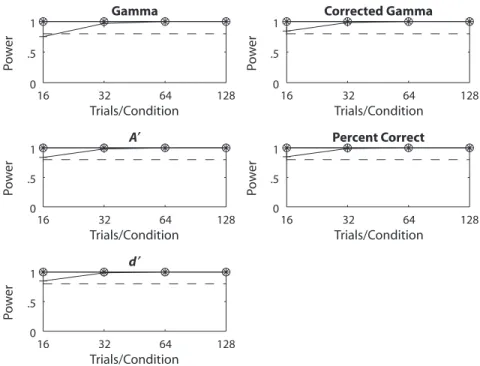
Gaussian distributions. Figure 12 shows the power results for γ, γC, A′, p(c),and log-linear adjusted d′, based on Gaussian distributions. Across all dependent measures, it is clear that power increases predictably with greater numbers of subjects and trials and with a larger effect size (the magnitude of the sensitivity difference, ddiff). Those parameter values determine power to a much greater ex-tent than does the choice of dependent measure. None-theless, some basic conclusions can be drawn about the relative performance of the single-point measures.
For small numbers of trials, A′ has the best power. Power is very similar for log-linear d′, γC, and percent correct, all of which have slightly more power than does γ. For all the measures, power is inversely related to sensitivity (d) in the weaker condition. This relationship occurs because, as
d increases, the hit rates in the two conditions are based on more extreme portions of the tails of the Gaussian distri-butions; as d rises, it takes an ever-larger shift of the distri-butions (ddiff) to create changes in H of equal magnitude.
Rectangular distributions. Figure 13 show the power of γ, γC, A′, p(c),and log-linear adjusted d′, respectively, based on rectangular distributions. As for the simulations based on Gaussian distributions, the primary determinants of power are the number of subjects, the number of tri-als, and the size of ddiff. All measures perform similarly, although some conclusions can be drawn. A′ performs particularly well when sensitivity (d) is low and there are few subjects and trials; γ has the lowest power under those the same method as that in our Type I error rate
simula-tions. For each subject, T trials were sampled at random from each of the target distributions as well as the lure distribution; these sampled values were compared with the decision criterion and resulted in “yes” responses if they exceeded that criterion. These “yes” responses were converted to a hit rate in each condition and a common false alarm rate for that subject.
For each combination of parameter values, we calculated a value of d′, A′, γ, p(c), and γC for each subject in each condition. As in the Type I error rate simulations, we ap-plied the log-linear, replacement, and discard methods of dealing with cases in which F 5 0 or H 5 1; these were applied to all the dependent measures. We also will report analyses based on the uncorrected data, where possible. One thousand simulated experiments were run for each set of parameter values; in each experiment, the subjects’ data were compared using a within-subjects t test. The number of significant t tests is the observed power for that dependent measure, correction method, and set of parameter values.
Results
As for the Type I error rate simulations, we will present results for the dependent measures as we judge research-ers to use them. So, we will show A′, p(c), γ, and γCin
d
diff0
k
d
σ
5
1/s
σ
5
1
Figure 10. parameter definitions for the Gaussian distribution power simulations.
d ddiff
0 k 1
Figure 11. parameter definitions for the rectangular distribu-tion power simuladistribu-tions.
16 32 64 128 0
.5
1 Gamma
Trials/Condition
Po
w
er
16 32 64 128
0 .5
1 Corrected Gamma
Trials/Condition
Po
w
er
16 32 64 128
0 .5
1 A′
Trials/Condition
Po
w
er
16 32 64 128
0 .5
1 Percent Correct
Trials/Condition
Po
w
er
16 32 64 128
0 .5
1 d′
Trials/Condition
Po
w
er
Figure 12. power simulations for all measures, assuming Gaussian distributions, true sensitivity d 5 1, k 5 1, zRoC slope 5 1.0, and 30 simulated subjects. Within each panel, the dashed line indicates power 5 .80, and the solid lines reflect values of ddiff: Symbols denote
ddiff 5 0.1 (plus sign), 0.3 (open circle), 0.5 (asterisk), 0.7 (x), and 0.9 (square).
16 32 64 128
0 .5
1 Gamma
Trials/Condition
Po
w
er
16 32 64 128
0 .5
1 Corrected Gamma
Trials/Condition
Po
w
er
16 32 64 128
0 .5
1 A′
Trials/Condition
Po
w
er
16 32 64 128
0 .5
1 Percent Correct
Trials/Condition
Po
w
er
16 32 64 128
0 .5
1 d′
Trials/Condition
Po
w
er
Figure 13. power simulations for all measures, assuming rectangular distributions, d 5 0.37, k 5 .85, and 30 simulated subjects. Within each panel, the dashed line indicates power 5 .80, and the solid lines reflect values of ddiff: Symbols denote ddiff 5 0.1 (plus sign),
viation from true values (Macmillan, Rotello, & Miller, 2004; Verde et al., 2006) and is an estimate of the area under the ROC.
When Distributions are Known
In some empirical situations, such as some perceptual categorization tasks, the stimuli are drawn from artificially created distributions (e.g., Ashby & Gott, 1988; Ratcliff, Thapar, & McKoon, 2001). In that case, the form of the underlying strength distributions is obviously known (and can be manipulated); selection of an appropriate sensitiv-ity measure is straightforward and follows the rules out-lined previously.
In other research domains, the form of the underlying strength distributions may be inferred from previous re-search in which ROC data were collected. Swets (1986a) summarized the form of the ROCs observed in a variety of basic and applied research domains. These ROCs were all consistent with Gaussian evidence distributions, al-though they sometimes indicated that the distributions were of equal variance (pure-tone detection), less often of unequal variance with a less variable target distribution (e.g., information retrieval systems, weather forecasting), and more often of unequal variance with a more variable target distribution (e.g., recognition judgments, decisions on radiological images).
As we have noted, no single-point sensitivity measure performs adequately when the underlying Gaussian distri-butions have different variances; in that case, some infor-mation about the ratio of target and lure standard devia-tions is necessary to accurately evaluate sensitivity. Worse, apparently small changes in the stimulus characteristics or task structure can result in changes to the form of the ROC. For example, shifting the task from detection of pure tones in noise to detection of signals that are white noise samples changes the ROC from equal-variance Gaussian to unequal-variance Gaussian (Green & Swets, 1966). In the domain of recognition memory, changing the nature of the lures can shift the form of the ROC from being consis-tent with Gaussian distributions (when lures are randomly related to targets) to being consistent with rectangular dis-tributions (when lures and targets differ in a single detail, such as their plurality [Rotello, Macmillan, & Van Tassel, 2000] or the side of the screen on which they are presented [Yonelinas, 1999]). Given that small experimental changes can affect the form of the ROC and that the form of the ROC determines which sensitivity measure is most appro-priate in a particular experimental task, ROCs are nearly always necessary for accurate interpretation of data.
When Distributions are unknown
What if the form of the underlying strength distribu-tions is completely unknown? In that case, a dependent measure that makes little to no assumption about the form of the distributions would be desirable. Two such purport-edly nonparametric measures have been proposed: γ and
A′. However, both measures have been shown to be para-metric (A′, Macmillan & Creelman, 1996; γ, Masson & Rotello, 2007). Our simulations contribute to the strong recommendation that these measures be avoided: Regard-conditions. When sensitivity and the number of trials are
high, log-linear d′ exaggerates the differences between conditions and provides greater power than do the other measures; γ has the lowest power under those conditions.
Discussion
Unlike our Type I error rate simulations, these power simulations indicate that all the dependent measures per-form fairly similarly. Power increases with subjects, trials, and the magnitude of the sensitivity difference between conditions; all of these effects are predictable. Power is also highest when sensitivity is low in the weaker tions, perhaps because performance in the stronger condi-tion is less constrained by a ceiling effect. Although the power simulations suggest that A′ is the best choice of dependent measure, regardless of the form of the underly-ing strength distributions, Figures 6 and 9 clearly indicate that this power does not come without a cost: the Type I error rates for A′ are unacceptably high.
ConCluSIonS anD ReCoMMenDaTIonS: unDeRSTanD youR DaTa
It is essential to choose a sensitivity measure that has properties that match the structure of the data to be ana-lyzed. Some measures, such as percent correct and the new γC, assume that the underlying strength distribu-tions are rectangular in form. In contrast, d′ assumes that the underlying strength distributions are equal-variance Gaussian. Our power simulations indicate that all of these measures perform well, given sufficient numbers of sub-jects and trials. However, the Type I error rate simulations demonstrate that application of an inappropriate depen-dent measure dramatically inflates the likelihood that an erroneous conclusion will be drawn about sensitivity differences between empirical conditions. To minimize Type I errors, if the data are truly drawn from rectangular distributions, percent correct or γC should be used. If the data are drawn from equal-variance Gaussian distribu-tions, d′ should be used, and the overall sensitivity levels should be kept at a moderate level to avoid Type I errors that stem from the correction for 0s and 1s. If the data are drawn from unequal-variance Gaussian distributions, no single-point measure consistently yields reasonable Type I error rates. The best one may do in that case is to estimate sensitivity using da (Simpson & Fitter, 1973) or Az (Swets & Pickett, 1982), if the relative magnitudes of the target (1/s) and lure standard deviations (1) are known or can be estimated from previous research. These values can be calculated as follows:
d
s zH szF
a = +
1 2 2
(
−)
1 2/(6) and
Az = da
Φ
2 , (7)
where Φ is the cumulative normal distribution function.
de-nal of Experimental Psychology: Learning, Memory, & Cognition,
32, 1133-1145.
Macmillan, N. A., & Creelman, C. D. (1996). Triangles in ROC space: History and theory of “nonparametric” measures of sensitivity and response bias. Psychonomic Bulletin & Review, 3, 164-170. Macmillan, N. A., Rotello, C. M., & Miller, J. O. (2004). The
sam-pling distributions of Gaussian ROC statistics. Perception &
Psycho-physics, 66, 406-421.
Masson, M. E. J., & Rotello, C. M. (2007). Bias in the Goodman–
Kruskal gammacoefficient measure of discrimination accuracy.
Manuscript submitted for publication.
Miller, J. (1996). The sampling distribution of d′. Perception &
Psy-chophysics, 58,65-72.
Murdock, B. B., & Ogilvie, J. C. (1968). Binomial variability in short-term memory. Psychological Bulletin, 70,256-260.
Nelson, T. O. (1984). A comparison of current measures of the accu-racy of feeling-of-knowing predictions. Psychological Bulletin, 95, 109-133.
Nelson, T. O. (1986a). BASIC programs for computation of the Goodman– Kruskal gamma coefficient. Bulletin of the Psychonomic
Society, 24, 281-283.
Nelson, T. O. (1986b). ROC curves and measures of discrimination ac-curacy: A reply to Swets. Psychological Bulletin, 100,128-132. Pollack, I., & Norman, D. A. (1964). A non-parametric analysis of
recognition experiments. Psychonomic Science, 1,125-126. Ratcliff, R., Sheu, C.-F., & Gronlund, S. D. (1992). Testing global
memory models using ROC curves. Psychological Review, 99, 518-535.
Ratcliff, R., Thapar, A., & McKoon, G. (2001). The effects of aging on reaction time in a signal detection task. Psychology & Aging, 16, 323-341.
Rotello, C. M., Macmillan, N. A., & Van Tassel, G. (2000). Recall- to-reject in recognition: Evidence from ROC curves. Journal of
Mem-ory & Language, 43, 67-88.
Schooler, L. J., & Shiffrin, R. M. (2005). Efficiently measuring rec-ognition performance with sparse data. Behavior Research Methods,
37,3-10.
Simpson, A. J., & Fitter, M. J. (1973). What is the best index of detect-ability? Psychological Bulletin, 80,481-488.
Snodgrass, J. G., & Corwin, J. (1988). Pragmatics of measuring rec-ognition memory: Applications to dementia and amnesia. Journal of
Experimental Psychology: General, 117,34-50.
Swets, J. A. (1986a). Form of empirical ROCs in discrimination and diagnostic tasks: Implications for theory and measurement of perfor-mance. Psychological Bulletin, 99, 181-198.
Swets, J. A. (1986b). Indices of discrimination or diagnostic accuracy: Their ROCs and implied models. Psychological Bulletin, 99, 100-117. Swets, J. A., & Pickett, R. M. (1982). Evaluation of diagnostic
sys-tems: Methods from signal detection theory. New York: Academic
Press.
Tanner, W. P., Jr., & Swets, J. A. (1954). A decision-making theory of visual detection. Psychological Review, 61, 401-409.
Verde, M. F., Macmillan, N. A., & Rotello, C. M. (2006). Measures of sensitivity based on a single hit rate and false alarm rate: The ac-curacy, precision, and robustness of d′, Az, and A′. Perception &
Psy-chophysics, 68, 643-654.
Verde, M. F., & Rotello, C. M. (2003). Does familiarity change in the revelation effect? Journal of Experimental Psychology: Learning,
Memory, & Cognition, 29,739-746.
Weaver, C. A., III, & Kelemen, W. L. (1997). Judgments of learning at delays: Shifts in response patterns or increased metamemory ac-curacy? Psychological Science, 8, 318-321.
Yonelinas, A. P. (1999). The contribution of recollection and famil-iarity to recognition and source-memory judgments: A formal dual-process model and an analysis of receiver operating characteristics.
Journal of Experimental Psychology: Learning, Memory, & Cogni-tion, 25, 1415-1434.
(Manuscript received April 6, 2007; revision accepted for publication September 14, 2007.)
less of whether the underlying distributions were rectangu-lar or Gaussian in form, both A′ and γ yielded unacceptably high Type I error rates across a wide variety of parameter values. Increasing the number of subjects or trials in the simulated experiment only exaggerates the problem, since the data converge on the wrong underlying model.
Conclusion
Unless the form of the underlying strength distributions are known and stable, either because they are constructed (e.g., Ashby & Gott, 1988) or because of consistent ROC results in prior research, an appropriate single-point de-pendent measure cannot be selected in a given experiment. In the absence of information about the distributions, the best option is to generate ROC curves. The shapes of ROC curves provide information about the form of the underlying distributions; thus, they allow more accurate calculation of sensitivity independently of bias. Given a design that supplies a reasonable number of data points per condition, the cost associated with producing ROCs is typically modest: They can usually be generated by asking subjects to make confidence ratings on each test probe, rather than binary decisions. Making that simple change will reduce Type I errors in the literature.
auTHoR noTe
C.M.R. is supported by Grant MH60274 from the National Institutes of Health, and M.E.J.M. is supported by a grant from the Natural Sciences and Engineering Research Council of Canada. We thank Neil Macmillan for many discussions of this research and for comments on a previous draft of the manuscript. Helena Kadlec and two anonymous reviewers were also extremely helpful. Correspondence concerning this article should be addressed to C. M. Rotello, Department of Psychology, Uni-versity of Massachusetts, Box 37710, Amherst, MA 01003-7710 (e-mail: [email protected]).
ReFeRenCeS
Ashby, F. G., & Gott, R. E. (1988). Decision rules in the perception and categorization of multidimensional stimuli. Journal of Experimental
Psychology: Learning, Memory, & Cognition, 14,33-53.
Balakrishnan, J. D. (1998). Some more sensitive measures of sensitiv-ity and response bias. Psychological Methods, 3,68-90.
Donaldson, W. (1993). Accuracy of d′and A′ as estimates of sensitivity.
Bulletin of the Psychonomic Society, 31,271-274.
Dougal, S., & Rotello, C. M. (2007). “Remembering” emotional words is based on response bias, not recollection. Psychonomic
Bul-letin & Review, 14,423-429.
Glanzer, M., Kim, K., Hilford, A., & Adams, J. K. (1999). Slope of the receiver-operating characteristic in recognition memory. Journal
of Experimental Psychology: Learning, Memory, & Cognition, 25,
500-513.
Goodman, L. A., & Kruskal, W. H. (1954). Measures of association for cross classifications. Journal of the American Statistical Associa-tion, 49, 732-764.
Green, D. M., & Swets, J. A. (1966). Signal detection theory and
psy-chophysics. New York: Wiley.
Hautus, M. J. (1995). Corrections for extreme proportions and their biasing effects on estimated values of d′. Behavior Research Methods,
Instruments, & Computers, 27,46-51.
Kadlec, H. (1999). Statistical properties of d′and β estimates of signal detection theory. Psychological Methods, 4,22-43.
Koriat, A., & Bjork, R. A. (2006). Mending metacognitive illusions: A comparison of mnemonic-based and theory-based procedures.