R E S E A R C H A R T I C L E
Open Access
Predicting volume of distribution with decision
tree-based regression methods using predicted
tissue:plasma partition coefficients
Alex A Freitas
1, Kriti Limbu
2and Taravat Ghafourian
2,3*Abstract
Background:Volume of distribution is an important pharmacokinetic property that indicates the extent of a drug’s distribution in the body tissues. This paper addresses the problem of how to estimate the apparent volume of distribution at steady state (Vss) of chemical compounds in the human body using decision tree-based regression methods from the area of data mining (or machine learning). Hence, the pros and cons of several different types of decision tree-based regression methods have been discussed. The regression methods predict Vss using, as predictive features, both the compounds’molecular descriptors and the compounds’tissue:plasma partition coefficients (Kt:p)–often used in physiologically-based pharmacokinetics. Therefore, this work has assessed whether the data mining-based prediction of Vss can be made more accurate by using as input not only the compounds’ molecular descriptors but also (a subset of) their predicted Kt:pvalues.
Results:Comparison of the models that used only molecular descriptors, in particular, the Bagging decision tree (mean fold error of 2.33), with those employing predicted Kt:pvalues in addition to the molecular descriptors, such as the Bagging decision tree using adipose Kt:p(mean fold error of 2.29), indicated that the use of predicted Kt:p values as descriptors may be beneficial for accurate prediction of Vss using decision trees if prior feature selection is applied.
Conclusions:Decision tree based models presented in this work have an accuracy that is reasonable and similar to the accuracy of reported Vss inter-species extrapolations in the literature. The estimation of Vss for new compounds in drug discovery will benefit from methods that are able to integrate large and varied sources of data and flexible non-linear data mining methods such as decision trees, which can produce interpretable models.
Keywords:Volume of distribution, Tissue partition, QSAR, QSPkR, Data mining, Machine learning, Decision tree, Pharmacokinetics, ADME
Background
Despite significant advances in pharmacology in the last decades, at present it is still very difficult to find (near)-optimal answers to the questions of how much, how often and for how long a drug should be given to a pa-tient, in order to maximize its therapeutic effect and minimize its adverse effects. This is especially important in drug discovery since, for a new drug candidate, a
poorly designed study with incorrect dose regimen can lead to misleading results which can prove very costly to the sponsor company when the product fails later in development.
In this context, this paper addresses an important pharmacokinetics problem: how to estimate the apparent volume of distribution of a drug in the human body at steady state (Vss), which is the volume of reference fluid (usually plasma) in which the drug appears to be dis-solved at steady state [1]. Although this apparent Vss has no physiological meaning, its estimation is important be-cause it predicts the drug’s plasma concentration for a given amount of drug in the body and it influences the drug’s half-life [2,3], which in turn is very important to
* Correspondence:[email protected] 2
Medway School of Pharmacy, Universities of Kent and Greenwich, Chatham, Kent ME4 4TB, UK
3
Drug Applied Research Centre and Faculty of Pharmacy, Tabriz University of Medical Sciences, Tabriz, Iran
Full list of author information is available at the end of the article
determine the correct dosage regimen that clinicians should prescribe to patients [4,5]. Hence, one needs to estimate or predict Vss using an in vivo, in vitro or in silicoapproach [6-9].
In vivoanimal models produce rich information about a drug’s pharmacokinetics properties, but they are a low-throughput approach which is very time-consuming and costly, as well as involving ethical issues. In vitro models are less time-consuming and less costly than in vivo ones, but they are still based on time-consuming and costly biological assays, being at best a medium-throughput approach. For a review and comparison of in vivo and in vitromethods for Vss prediction, see e.g. ref. [10].
In silico models are theoretical models that lack the experimentally-derived rich information associated with in vivo or in vitro models, but they are a very high-throughput approach, which is much less time-consuming and costly thanin vivo andin vitroapproaches. Hence, the results of an in silicomodel can be used to suggest which chemical compounds should have a higher prior-ity to be further tested by the more expensive but more accuratein vivoandin vitroexperiments. In addition to much smaller time and cost requirements, in silico models have the advantages that they can be directly generated with human data and can even be used to evaluate the pharmacokinetics of compounds which have not been synthesized yet, which is not possible within vivoandin vitroexperiments.
This work is based on the in silico approach, using data mining (or machine learning) methods to build models that predict the Vss using the properties of mo-lecular structures of chemical compounds as the model features. Such a modeling approach is generally known as Quantitative Structure-Activity Relationship (QSAR) ap-proach, with the special QSAR case here being the Quanti-tative Structure-Pharmacokinetic Relationship (QSPkR) modeling [11,12]. More precisely, we use two types of data mining methods – mainly decision tree-based regression methods, but also a feature selection method (see Methods section)–to produce QSPkR models that predict the Vss of chemical compounds.
Conventional QSPkR modeling methods for predicting Vss normally use, as features, a large set of physico-chemical or molecular descriptors, most of which are calculated by specialized software. The use of such phys-icochemical descriptors as potential predictors of Vss makes sense because, broadly speaking, the Vss of a drug is mainly determined by its nonspecific binding to plasma and tissue components, rather than its specific pharmacophore, and such nonspecific binding is to a large extent determined by the drug’s physicochemical properties [4,13,14]. In addition, binding to the pharma-cological target is considered to have relatively little
importance for predicting Vss, since the level of target expression is usually low [15].
As an alternative to building QSPkR models for pre-dicting Vss based on physicochemical drug properties, several studies use a physiologically-based pharmacokin-etics (PBPK) approach for predicting the Vss of a drug based on its tissue:plasma partition coefficients (Kt:p),
where a compound’s Kt:p is its concentration ratio
be-tween a tissue and plasma at steady state. The basic idea is to determine the Kt:pvalue for each of the major
tis-sues in the body where a drug can be present in signifi-cant concentration and calculate the Vss for the whole body as a function of the sum of the product of Kt:pand
tissue volume for all those tissues, using (variations of ) the following equation [16,17]: Vss=Vp+Ve× (E:P) +Σt (Vt×Kt:p), where Vp, Ve and Vt are the volumes of
plasma, erythrocyte and tissue, respectively, E:P is erythrocyte-to-plasma partition coefficient, and Kt:p is
the tissue:plasma partition coefficient for tissue t. Note that this equation refers to Kt:p coefficients based on
total concentrations in tissue and plasma, but one could use instead coefficients referring to the unbound drug concentrations [18,19].
The use of such tissue-composition-based equations to predict Vss has the advantage of providing a model with a clear interpretation about where drugs are being dis-tributed; but it introduces the problem of obtaining the Kt:p coefficients for a number of tissues, for each
drug. These are typically obtained via in vivoorin vitro experiments (whose limitations were briefly mentioned earlier) in animals, as they are difficult to be determined in humans [20]. Bothin vitroandin vivoapproaches are based on the measurement of drug concentration in the tissues and in the plasma at equilibrium or steady state. The model animals used in these studies are most often rat. In fact, rat is one of the most commonly used verte-brate in the estimation of pharmacokinetic parameters by interspecies scaling [21]. Due to the difficulty of obtaining experimental Kt:p values for a large number of
drugs, an alternative approach consists of predicting Kt:p
values and then using those predicted values to predict the Vss of a large number of compounds. This is essen-tially the approach that we propose here.
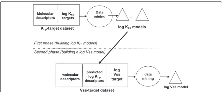
More precisely, we propose a new QSPkR approach consisting of two phases. In the first phase we obtained, from the literature, experimentally derived Kt:p values
for a relatively small set of 110 compounds, and used that dataset to build QSPkR models predicting Kt:p
values for different tissues based on molecular descrip-tors. In the second phase, we used the models built in the first phase to predict Kt:pfor a larger set of 604
com-pounds, and then used the predicted Kt:p values as
phase, we used the Vss dataset made available by Obach et al. [14]. This dataset has the advantages of being manu-ally curated, being relatively large and containing only data collected from intravenous studies–which avoids the un-certainties about the degree of bioavailability in common routes of administration, like oral administration.
It is important to note that the dataset used here has a very diverse set of compounds, unlike other studies in the literature that focus on relatively small subsets of Obach et al.’s dataset–see, e.g., ref. [5,22]. On one hand, this large compound diversity makes it difficult to dis-cover a model that predicts Vss with a high accuracy; but on the other hand the models produced in this study have a wider domain of applicability than other Vss models more specialized for certain classes of drugs. We will elaborate on this issue in the Discussion section.
The main contribution of this paper is to investigate whether or not the data mining-based prediction of the Vss of chemical compounds can be made more accurate by using as input not only the compounds’molecular de-scriptors but also computationally predicted tissue:plasma partition coefficients (Kt:pvalues) for those compounds for
a (sub) set of tissues. A secondary contribution of this work is that we discuss the pros and cons of several differ-ent types of decision tree-based regression methods and report the results of experiments comparing their predict-ive accuracy when building models to predict Kt:pand Vss.
To our knowledge, these two contributions have not been reported yet in the pharmacokinetics or QSAR literature.
Methods
The main dataset used in this research is a dataset con-taining 604 compounds with Vss values at steady state in humans, obtained from Obach et al.’s work [14], and our ultimate goal is to build models that predict human Vss for compounds in that dataset based on molecular de-scriptors and tissue:plasma partition coefficient (Kt:p)
de-scriptors, as mentioned in the Introduction. However, the experimental Kt:p values for different human tissues
are unknown for the large majority of those compounds. Hence, in this study we propose a two-phase approach for building models predicting human Vss in steady state. In the first phase we build QSPkR models for pre-dicting log Kt:pvalues for different tissues based on
mo-lecular descriptors; whilst in the second phase we used the predicted log Kt:p values as descriptors, in addition
to molecular descriptors, to build QSPkR models pre-dicting log Vss. These two phases are described in more detail next.
The first phase of the proposed approach–building QSPkR models for predicting Log Kt:p
Experimentally derived Kt:p values were available in the
literature for a number of rat tissues for 110 compounds
(see Additional file 1 for the dataset, including the ori-ginal references for the data). ACDlabs logD 12.0 and MOE (Molecular Operating Environment) 2011 software were used to calculate about 300 molecular descriptors for each of these compounds, as described in detail in ref. [23]. This dataset was created with rat tissue Kt:p,
ra-ther than human tissue Kt:p, because there is
substan-tially more data for the former than for the latter in the literature. Hereafter, we refer to that created dataset as the Kt:p-target dataset. In essence, it included several
types of drugs, such as NSAIDs, anticonvulsants, sulfo-nylureas, benzodiazepines, beta blockers, antipsychotics and some antibiotics such as cephalosporins, fluoroqui-nolones, tetracyclines, etc. Then, we applied data mining methods (described later) to the Kt:p-target dataset in
order to build a regression-type model for predicting the log Kt:p(where the log is in base 10) for each of 13
dif-ferent tissues whose data is included in the Additional file 1, based on the molecular descriptors of the com-pounds. This process is summarized in graphical form in the top half of Figure 1.
Note that, for most compounds in the created dataset, there is a large proportion of missing values for the log Kt:p of most tissues (See Additional file 1). For one of
the tissues, namely pancreas, only 3 compounds in the dataset have a known log Kt:p value, and so no attempt
was made to build a regression model predicting pan-creas log Kt:p values from so few compounds. For each
of the other tissues, we tried to build regression-type models predicting the log Kt:pvalue for that tissue. This
generated 13 different regression-type problems, each characterized by a different target (dependent, or re-sponse) variable, representing the log Kt:p of a different
tissue, and a different (but overlapping) set of com-pounds. On the other hand, the set of descriptors (fea-tures, or independent variables) used to build the models was the same in all 13 regression problems, con-sisting of about 300 molecular descriptors.
In each of those regression-type problems, all com-pounds with known log Kt:p value for the target tissue
were used to build and validate models predicting the target tissue’s log Kt:p value. For each tissue, we built
several QSPkR models predicting that tissue’s log Kt:p
value using different types of decision tree-based regres-sion methods (described later). The error rate associated with each method was measured by a 10-fold cross-validation procedure, which works as follows [24]. First, the Kt:p-target dataset was randomly divided into 10
predicting log Kt:pfor each tissue is chosen as the model
produced by the method with the lowest MAE. The best model built for each tissue can then be used to predict that tissue’s log Kt:pvalue in the Vss-target dataset. Note
that the use of a cross-validation procedure is not shown in Figure 1 in order to keep the figure simple.
It is important to note that, when building a model to predict a certain tissue’s log Kt:p, the log Kt:ps of other
tissues are not used as descriptors. This restriction was implemented because a model built from the Kt:p-target
dataset is used later to predict a tissue’s log Kt:pvalues in
the Obach et al.’s dataset, where other tissues’ log Kt:p
values are unknown.
The second phase of the proposed approach–building QSPkR models for predicting Log Vss
In this phase we used a larger set of 604 compounds and corresponding steady state Vss values in humans ob-tained from ref. [14]. The dataset published by Obach et al. consists of Vss values for 665 compounds. In this study, some of the compounds were removed because their molecular descriptors could not be calculated. This was the case for compounds containing metals, or other salts, or permanently charged compounds such as qua-ternary ammoniums. We also removed from the initial dataset all compounds that were included in our Kt:p
-target dataset. As a result, the final version of the dataset used in our experiments has 604 compounds. We refer to this dataset as the Vss-target dataset hereafter. As mentioned earlier, the log Kt:pvalues of different tissues
are unknown for the large majority of compounds in the Vss-target dataset. Hence, we used the best regression
models built in the first phase (i.e. the best model for each tissue) to predict the set of tissues’ log Kt:p values
for the compounds in this dataset. Again, ACDlabs logD 12.0 and MOE (Molecular Operating Environment) 2011 software were used to calculate about 300 molecu-lar descriptors for each compound in the Vss-target dataset [23]. Then we applied data mining methods to the Vss-target dataset in order to build regression models predicting log Vss in steady state in humans (where the log is in base 10), using as descriptors both the set of calculated molecular descriptors and the pre-dicted log Kt:p values. We built models predicting log
Vss, rather than Vss, because Vss has a very skewed dis-tribution, with relatively few compounds having very high Vss values. This process is summarized in graphical form in the bottom half of Figure 1. In both phases, the regression models are expressed in the form of decision trees, as will be explained next.
An overview of the decision tree-based regression methods used in this work
The type of regression method used in both the previ-ously described phases of the proposed approach was decision-tree building algorithms. In essence, this type of method builds a decision tree by recursively partitioning the set of compounds in the training set, as follows. First, it considers all training set compounds, selects the descriptor that is the best predictor of the value of the target variable (a tissue’s log Kt:pin the first phase or log
Vss in the second phase, in this work), adds the selected descriptor to the tree (as its root node), and partitions the training set based on the values of the selected
descriptor. In this context, the best predictor is the pre-dictor that partitions the data in a way that each of the resulting nodes has the minimum possible variance in the values of the target variable. Typically, in the case of numerical variables, this involves creating two training set partitions, one with compounds satisfying the condi-tion dsel≤t and the other with compounds satisfying dsel>t, where dsel is the selected descriptor and t is a threshold automatically chosen by the algorithm. Next, the same process of selecting the best descriptor, adding it to the tree and further partitioning the current set of compounds is applied to each of the just-created parti-tions (nodes). This process is recursively applied until a stopping criterion is satisfied for each partition, e.g. when the variance of the value of the target variable for the compounds in the current partition is below a pre-defined threshold, in which case a leaf node (terminal node) is created for that partition. The result of this process is a decision tree, where internal (non-leaf ) nodes contain names of descriptors, the edges coming out from a node contain conditions likedsel≤tordsel> t, and each leaf node predicts the value of the target variable for the compounds that have the descriptor values associated with the edges in the path from the root node to that leaf node. The leaf node’s prediction can be performed in different ways, associated with dif-ferent types of decision trees, as discussed later.
We chose this paradigm of decision tree-based regres-sion methods for several reasons. First, they produce graphical models that can be potentially comprehensible and interpretable by users [24-27]. This is in contrast to methods such as support vector machines and artificial neural networks, which produce models that are a kind of “black box”, being hardly interpretable by users. Sec-ond, they produce models capturing non-linear relation-ships in the data, instead of simply modeling only linear relationships, like traditional linear regression models often used in QSPkR studies. In addition, the paradigm of decision tree methods is broad enough to include several different types of decision trees (with different types of structures) for regression, which gives us more opportunities to try to find the best type of tree struc-ture for our target regression problem. More precisely, in this work we compare the effectiveness of several types of decision tree-based model structures for regres-sion, as follows.
(Conventional) regression trees
This type of decision tree structure has been popularized by the well-known CART (Classification and Regression Tree) algorithm [28]. In a regression tree, in each leaf (terminal) node, the log Vss value predicted for a new compound reaching that node is given by the mean of log Vss values over all the training set compounds that
belong to that node. The main advantages of such regres-sion trees are their simplicity and easy interpretation; i.e., each leaf node directly provides a predicted log Vss value, unlike the case of model trees, discussed next.
Model trees
This is a more sophisticated type of decision tree for re-gression. In a model tree, in each leaf node, the log Vss value predicted for a new compound reaching that node is given by a multivariate linear regression model built from the training set compounds that belong to that node [29]. Note that, at each leaf node, the linear model contains only descriptors that occur in tree nodes in the path from the root to the current leaf node or descrip-tors that occur in linear models somewhere in the sub-tree containing the current leaf node. After building such a linear model using standard linear regression techniques, the linear model can be simplified by remov-ing irrelevant variables, usremov-ing a greedy search procedure that tries to improve the model’s estimated error rate. Hence, a model tree performs embedded feature selec-tion at two levels, i.e., at the level of internal (non-leaf ) nodes and at the level of leaf nodes. The model tree ap-proach is much more flexible than the conventional lin-ear regression approach of building a single (global) linear model from the entire training set, because the latter makes the strong assumption that all the com-pounds have the same relationship between features and log Vss. By contrast, a model tree recognizes that differ-ent linear equations might describe well the relationship between features and log Vss for different subsets of compounds. Hence, in theory model trees can better adapt their structure to a diverse set of compounds, such as the Vss-target dataset used in this work. On the other hand, model trees tend to be more difficult to interpret than regression trees, since a single model tree can have a large number of linear equations (each with tens of de-scriptors) in its leaves. We will discuss the interpretation of model trees later.
If-then regression rules
estimated accuracy) and creates a rule corresponding to the path from the root to that leaf node, throwing away the rest of the tree. By iteratively repeating this proced-ure, it builds a set of modularIf-Then rules, rather than a decision tree.
Bagging
Bagging (which stands for Bootstrap Aggregation) con-sists of an ensemble (or set) of decision trees, where dif-ferent decision trees in the ensemble are produced by different random samplings (different bootstrap samples) of the original training set [31]. When we need to pre-dict the log Kt:p or log Vss of a new compound, a
pre-dicted value is computed by each tree in the ensemble, and the predictions are averaged to give the ensemble’s prediction. Bagging can be used to produce a set of re-gression or model trees. In this work, all the trees in the ensemble produced by Bagging are model trees, since this type of decision tree produced somewhat better re-sults than regression trees in our preliminary experi-ments. Bagging has the advantage of increasing the robustness of the model (reducing the variance of its predictions), by comparison with using a single decision tree, since its prediction is an average of the prediction of many models. However, Bagging has the disadvantage of producing a more complex model, which is consider-ably more difficult to interpret than a single decision tree. We will also discuss the interpretation of a Bagging model later.
Correlation-based feature selection (CFS) with genetic search
From a feature selection perspective, all the previously described decision tree-based regression methods per-form “embedded feature selection”, in the sense that a decision tree is built by selecting the“best”feature to be used in each node of the tree, and normally only a proper subset of the input features is selected to occur in some tree node. A different type of feature selection method performs feature selection in a preprocessing phase, before running the decision tree building algo-rithm –or any other type of classification algorithm for that matter. It is often possible to achieve better predict-ive accuracy using a two-stage approach, where we first use a preprocessing feature selection method and then apply a decision tree building algorithm to the features selected in the first stage. For evidence that this ap-proach can improve predictive accuracy over using just a decision tree building method, see e.g. Newby et al.’s work [32]. Hence, in this work we also tried to use one type of preprocessing feature selection method, namely genetic search-based CFS, which was also successfully used by Newby et al.. In essence, this method uses a genetic algorithm as a search method in the space of candidate feature (descriptor) subsets, and evaluates the
quality of each candidate feature subset using a“fitness” (evaluation) function that considers two criteria: the cor-relation between features in that candidate subset and the target variable, and the redundancy among features in that candidate subset. The genetic search is used to find a feature subset that maximizes that correlation and minimizes that redundancy. For a review of the CFS method, see ref. [33], and for a review of genetic search applied to feature selection, see e.g. ref. [34].
Results
Results for the regression models predicting each Tissue’s Log Kt:pvalues
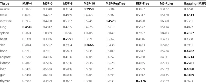
Table 1 shows, for each tissue, the mean absolute error (calculated by 10-fold cross-validation [24]) in the pre-diction of log Kt:p by each regression method, in our
Kt:p-target dataset. As discussed in the Methods section,
we investigated the use of different types of decision tree-based regression methods. More precisely, the first four regression methods in Table 1 are variations of model trees built by the M5P algorithm in WEKA [29], where each variation used a different value of the param-eter ‘minNumInstances’ (the minimum number of in-stances (compounds) to allow at a leaf node), namely the value 4, 6, 8 or 10, as indicated in the column headings. The column heading M5P-RegTree refers to the M5P version buildingregression trees, rather than model trees. REP-Tree is a method that produces a regression tree and was designed particularly to be fast, which may however lead to some reduction in its predictive accur-acy, by comparison with other decision tree methods. M5-Rules is an M5P version that produces a model con-sisting of a list of If-Then regression rules, rather than regression trees [30]. The Bagging-M5P method [31] produces a set of M5P model trees and predicts, for a new compound, the value of a target variable that is an average of the values predicted by the individual model trees. The number of trees produced is a parameter, for which we used the default value of 10 in WEKA.
In Table 1, for each tissue, the smallest Mean Absolute Error (MAE) – among the 8 regression methods – is highlighted in bold. As expected, there is no single re-gression method that is the best across all tissues, but overall the Bagging-M5P method is the most successful one. It obtains the smallest MAE in 7 out of the 13 tis-sues. Recall, however, that our goal is not to select the best regression method overall, but rather to select the best regression method to predict the log Kt:p value for
each tissue. The best model built for each tissue was then used to predict that tissue’s log Kt:p value for all
compounds in the Vss-target dataset, where those pre-dicted log Kt:pvalues are used as descriptors (in addition
As can be seen in Table 1, the value of the best (smal-lest) MAE for each tissue varies from 0.2176 and 0.2281 for the log Kt:p’s of thymus and kidneys, respectively, to
0.7857 for the log Kt:p of spleen. Given this significant
variability in the MAE values, one could wonder whether just a subset of the models having relatively small MAEs (e.g., values below a certain threshold) should be used for predicting the tissue log Kt:pvalues to be used as
descrip-tors in the Vss-target dataset, whilst other tissues’log Kt:p
values (with large MAEs) should be ignored. However, this would introduce the problem of how to determine which MAE values are small enough for their corresponding pre-dicted log Kt:pto be reliably used as descriptors in the
Vss-target dataset. A predefined threshold would be an ad-hoc solution. In addition, the MAE value by itself seems not to be an effective measure of the usefulness of a predicted log Kt:pvalue, because the predicted values will be used as
descriptors for building models predicting log Vss in the Vss-target dataset, which is a regression problem very dif-ferent from the problem of building the models reported in Table 1.
Hence, once the best model predicting log Kt:p has
been selected for each tissue based on the results shown in Table 1, the decision about which of those models will be used as descriptors should be made by directly taking into account the predictive performance of each pre-dicted log Kt:pdescriptor in log Vss models. In our case,
this is naturally done by taking advantage of the fact that the decision tree-based regression methods used to pre-dict log Vss perform an embedded ‘descriptor selection’ (or feature selection) procedure as part of the decision tree building process –recall that only descriptors con-sidered relevant for predicting the target variable are included in the decision tree. That is, we let the decision
tree-based regression methods use, as input descriptors, the set of predicted log Kt:p values for (almost) all the
tissues – in addition to the aforementioned large set of molecular descriptors. Then the tree-building algorithm automatically decides which of those predicted log Kt:p
descriptors – as well as which molecular descriptors – are relevant enough to be included in the decision tree predicting log Vss. Out of the 13 tissues shown in Table 1, there is only one whose best log Kt:p-predicting
model was not used to fill in the corresponding descrip-tor values in the Vss-target dataset, namely the model for intestine. This is because the best model for this tis-sue’s log Kt:pconsists of a degenerated decision tree
hav-ing only one leaf node, which predicts the same value of intestine log Kt:pfor all new compounds, making it
use-less as a descriptor.
Results for the regression models predicting Log Vss In order to evaluate the predictive performance of models predicting log Vss, the Vss-target dataset was randomly divided into two sets. One set, with 402 com-pounds, is used as the model selection set; whilst the other set, with the remaining 202 compounds, is used as an external validation set. To perform model selection, each of the aforementioned decision tree-based regres-sion methods was applied to the model selection set, using 10-fold cross-validation. Then the best model – i.e., the one with smallest mean absolute error (MAE)– is selected, and that model is used to predict log Vss for the compounds in the external set. We emphasize that the compounds in the external set were not used in the model selection set (nor in the Kt:p-target dataset),
i.e., the external set compounds were not used in any way to build or select models, and so the predictive Table 1 Mean Absolute Error (calculated by 10-fold cross-validation) in the prediction of log Kt:pvalue by different decision tree-based regression methods, for each tissue, in Kt:p-target dataset (with 110 compounds)
Tissue M5P-4 M5P-6 M5P-8 M5P-10 M5P-RegTree REP-Tree M5-Rules Bagging (M5P)
muscle 0.3029 0.3040 0.3164 0.2950 0.3384 0.3857 0.3172 0.3228
brain 0.4695 0.4797 0.4869 0.4768 0.5387 0.5347 0.5170 0.4613
intestine 0.5939 0.4700 0.5337 0.5245 0.4523 0.4698 0.6060 0.5361
lung 0.4549 0.4812 0.4755 0.4776 0.5710 0.5522 0.5114 0.4822
spleen 0.9824 1.0069 1.0276 1.0206 0.8149 0.7997 0.8783 0.7857
heart 0.3391 0.3076 0.2991 0.3321 0.3562 0.4116 0.3723 0.3358
skin 0.2844 0.2752 0.2954 0.2666 0.3436 0.3433 0.2782 0.2961
bone 0.6210 0.7101 0.5893 0.5735 0.5109 0.5847 0.5724 0.4762
adipose 0.3581 0.4106 0.4186 0.4005 0.4557 0.5268 0.4031 0.3214
kidneys 0.2848 0.2706 0.2756 0.2736 0.3226 0.4035 0.2913 0.2281
liver 0.5495 0.5634 0.5036 0.5091 0.4925 0.5569 0.5879 0.4608
gut 0.6484 0.6134 0.6056 0.4905 0.4695 0.3912 0.4135 0.3169
performance in the external set represents a fair measure of the generalization ability of the used decision tree-based regression models.
Table 2 shows the MAE–calculated by 10-fold cross-validation–in the prediction of log Vss in the model se-lection dataset. This table has 3 columns with results. The first one reports results for each regression method when using, as input descriptors, both the set of 12 tis-sue log Kt:ps whose values were predicted by the
corre-sponding best model in Table 1 and a set of about 300 molecular descriptors – as explained earlier. The next column reports the results for each regression method when using, as input descriptors, only the set of molecu-lar descriptors. Hence, in those experiments the pre-dicted tissue log Kt:ps were not used as descriptors for
predicting log Vss, providing us with a baseline set of ex-periments against which we can measure the influence of using predicted tissue log Kt:ps as descriptors.
The last column in Table 2 reports the results of another set of experiments involving a two-step feature selection approach, as follows. First we apply a feature (descriptor) selection method to the dataset containing, as input de-scriptors, both the set of 12 tissue log Kt:ps whose values
were predicted by the corresponding best model in Table 1 and the large set of molecular descriptors. The feature se-lection method used was Correlation-based Feature Selec-tion (CFS) with genetic search (see Methods secSelec-tion). Out of the 56 descriptors selected by the CFS method, only two are predicted log Kt:pdescriptors, namely the log Kt:p
for adipose tissue and thymus. In the second step, the 56 descriptors selected by CFS are used as input by a decision tree-based regression method. Note that in the first step a descriptor subset is selected by CFS in a preprocessing phase, independent from the regression method; and in the second step the embedded descriptor selection pro-cedure of the regression method further selects a (usually
smaller) subset of relevant descriptors. This kind of two-step feature selection approach has also been successfully used to build other types of QSPkR models [32].
In Table 2, the best result (smallest MAE) for each type of descriptor set is highlighted in bold. As can be observed in the Table, the M5P algorithm generating a regression tree produced the best model when using the first type of descriptor set, whilst Bagging produced the best models when using the other two types of descriptor sets.
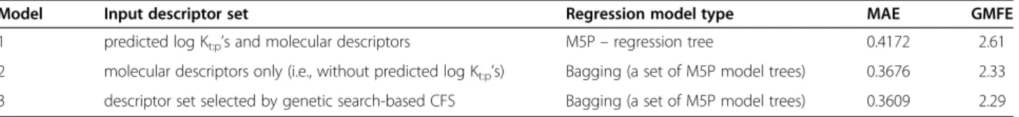
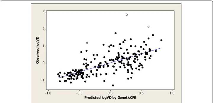
Finally, for each of the three types of descriptor sets, the best model identified in Table 2 was used to predict the log Vss of all compounds in the external set. The re-sults are shown in Table 3. The Geometric Mean Fold Errors (GMFEs) shown in that table were calculated as: GMFE = antilog10(MAE) [3]. The GMFE measure has the
advantage of being less affected by extreme outliers, by comparison with the coefficient of determination (which measures the quadratic error) [35]. In order to interpret the GMFE measure, note that a model with a GMFE of 2 makes Vss predictions which are on average twofold off– i.e., 100% above or 50% below the true Vss value.
As can be observed in Table 3, the approach of using as descriptors both the predicted log Kt:p values for 12
tissues and a large set of molecular descriptors (model 1) was not successful, by comparison with the baseline approach of using as descriptors only a large set of mo-lecular descriptors (model 2). The former approach ob-tained a GMFE of 2.61, versus a GMFE of 2.33 for the baseline approach. However, when the more sophisti-cated approach of selecting descriptors with both the genetic search-based CFS and the decision tree method was used (an approach that also used predicted log Kt:p
values as descriptors), a small improvement over the baseline approach was obtained, with the GMFE being slightly reduced from 2.33 to 2.29. AT-Test of mean dif-ference with a 95% confidence interval indicated the difference between the prediction errors was not statisti-cally significant (confidence interval of (−0.031, 0.017) and p = 0.577). Despite this, the significance of log Kt:p
in the prediction of Vss was very clear based on the fact that all the models where log Kt:p parameters were
in-cluded as input parameters (Model 1 and all the model trees making up Model 3) used a log Kt:p parameter as
the most important descriptor (see model interpretations in the next two sections).
The fact that the approach of using the predicted log Kt:p values as descriptors without running genetic
search-based CFS (model 1) led to a higher GMFE than the baseline may be due to a number of factors. One ex-planation may be the two phase approach adding a level of uncertainty due to the use of predicted, as opposed to the experimentally measured, Kt:pvalues. Despite the
ad-vantages of using tissue distribution from a mechanistic
Table 2 Mean Absolute Error (MAE)–calculated by
10-fold cross-validation–in the prediction of log Vss by each regression method, in model selection dataset (with 402 compounds)
Regression method
MAE (logVss)
Descriptor set includes predicted log Kt:p’s
Descriptor set without predicted log Kt:p’s
Descriptor set selected by genetic CFS
M5P-4 0.3891 0.3698 0.3739
M5P-6 0.3823 0.3665 0.4003
M5P-8 0.4715 0.3616 0.3847
M5P-10 0.4751 0.3658 0.3763
M5P-RegTree 0.3689 0.3772 0.3782
REPTree 0.3824 0.4330 0.3974
M5Rules 0.3911 0.3843 0.3836
point of view, the use of predicted tissue to plasma parti-tion coefficients can subject the model to the errors as-sociated with Kt:p prediction. This is in addition to the
experimental error associated with thein vitroorin vivo measurements of partition coefficients [36], which is es-pecially variable for basic lipophilic compounds [37]. Therefore, it is essential to ascertain the quality of pre-dicted Kt:p values for the compounds in Vss-target data
set. It is usually noted that prediction by a QSAR model is reliable only to compounds that are similar to the training set compounds [38]. In this case, the com-pounds in the Vss-target dataset need to be within the molecular descriptor boundaries of the Kt:pdataset.
Here, we used a descriptor range-based approach to identify compounds within or outside the molecular de-scriptor space. Since only one log Kt:p parameter has
been used in the set of model trees built by M5P in model 3 in Table 3, namely Kt:p for the adipose tissue,
the descriptor boundary was investigated only for this parameter. First, the set of descriptors that was used for the prediction of adipose tissue’s log Kt:pwere identified.
This set contains 16 descriptors. Then, compounds in the Vss validation set that have at least one descriptor value outside the descriptor values of the Kt:p dataset
were identified. Out of 202 compounds in the Vss valid-ation set, 43 compounds (21%) were identified as falling outside the range of the descriptor values of the Kt:p
data-set. The average error for all validation set compounds and the validation set excluding the 43 compounds were found to be similar (2.29 for all compounds vs 2.34 for compounds that are within the descriptor space). The rea-son for a very similar error for the validation set com-pounds within and those outside the descriptor range could be due to the source of Vss error being other param-eters than the uncertainties of log Kt:pprediction. For
ex-ample, one important observation for the compounds showing high Vss prediction error (by all methods) is that the large majority of these compounds have a relatively extreme (very high or very low) Vss value, which seems to be the main reason for their large errors. In other words, these major outliers are“prediction outliers”rather than“descriptor outliers”. As further evidence, a compari-son of the compounds that are outside the descriptor boundary with those that are within the descriptor range shows that in general compounds with similar chemical
and pharmacological nature can be found in both groups. For example, three out of nine cephalosporins and one out of seven penicillins and two out of four quaternary ammonium muscle relaxants are outside the domain with the remaining similar structures within the boundary.
To further evaluate the reliability of the predicted log Kt:pfor adipose tissue for the prediction of Vss, we
per-formed a sensitivity analysis to investigate how uncer-tainty in the regression for adipose tissue’s log Kt:p
prediction affects the prediction of Vss. More precisely, we performed a controlled experiment where we artifi-cially introduced 10% of noise to the predicted adipose tissue’s log Kt:p, as follows. For each compound in the
entire Vss-target dataset (including both the training (model selection) and external datasets), the value of the predicted adipose tissue’s log Kt:pdescriptor in that
com-pound was modified by adding or subtracting 10% of the current descriptor value, where the decision to perform addition or subtraction was made at random. This pro-cedure was repeated five times, varying the random seed used to decide if the 10% of noise was added or sub-tracted to each compound, which led to 5 new modified versions of the Vss-target dataset. For each of these 5 modified Vss-target datasets, we ran again the Bagging M5P regression algorithm and measured its geometric mean fold error (GMFE), averaging the results over the 5 runs. This procedure led to a GMFE or 2.35, which should be compared to the GMFE of 2.29 obtained by Bagging using the original predicted adipose tissue’s log Kt:p
de-scriptor values (without any extra artificial noise) – as reported in Table 3. Hence, a small degree of noise added to the predicted adipose tissue’s log Kt:p only moderately
affected the prediction of Vss, giving us more confidence in the relevance of this tissue’s log Kt:pto predict Vss.
In order to further understand the effect of this small degree of noise in the predictive power of the predicted adipose tissue’s log Kt:p descriptor, we also computed
the frequency of occurrence of this descriptor in the root node of the model trees built by Bagging M5P. Recall that a model tree’s root node contains the most relevant descriptor for predicting Vss. When using the original predicted adipose tissue’s log Kt:p descriptor
values (without any extra artificial noise), that descriptor occurs as the root node in all the 10 model trees built by Bagging. On the other hand, using the predicted adipose Table 3 Mean Absolute Error (MAE) and Geometric Mean Fold Error (GMFE) calculated for each combination of input descriptor set and the best regression model for that descriptor set, when predicting log Vss for all compounds in the external set (with 202 compounds)
Model Input descriptor set Regression model type MAE GMFE
1 predicted log Kt:p’s and molecular descriptors M5P–regression tree 0.4172 2.61
2 molecular descriptors only (i.e., without predicted log Kt:p’s) Bagging (a set of M5P model trees) 0.3676 2.33
tissue’s log Kt:pdescriptor values with 10% of noise, this
descriptor occurs as the root node, on average, in 8.6 of the 10 model trees. So, again the decrease in the rele-vance of this descriptor was not great; it is still the most relevant descriptor overall in the set of model trees built by Bagging, even with 10% noise added to its value, which further reinforces our confidence in the predictive power of this descriptor.
Distribution coefficients are the main factors control-ling the Vss of drugs. However, here we used data for rat Kt:p, rather than human Kt:p, when building models
pre-dicting log Kt:p. As mentioned earlier, this was due to
the availability of more rat Kt:p data than human Kt:p
data in the literature, but clearly there are species differ-ences that lead to different values of Kt:p for rats and
humans [6,39]. In addition, even when using rat Kt:p
data, the number of compounds with known log Kt:p
value available for some tissues (i.e. data required to build the model for those tissues) was still relatively small, which also limited the predictive accuracy that could be achieved by the log Kt:p models. However, the
fact that the third approach in Table 3, selecting descrip-tors (including predicted log Kt:p values) using both the
genetic search-based CFS and the decision tree method, achieved the best results overall suggests that at least some tissue(s)’ log Kt:p(s) were predicted well enough
and were correlated with Vss strongly enough to im-prove the predictive accuracy, by comparison with the baseline approach of not using predicted log Kt:pvalues.
Hence, a natural question to ask is whether the de-scriptors representing predicted log Kt:pvalues are often
selected to be included in the decision tree models, in the case of the first and third approaches in Table 3. This question is discussed in the next two sections. Note that the question is not valid in the case of the second approach, where predicted log Kt:p values are not used
as descriptors.
Interpreting the regression tree for predicting Vss built by M5P from predicted Kt:pand molecular descriptors
The best model built by M5P when using as input the 12 predicted log Kt:pdescriptors for different tissues is a
regression tree where log Kskin:plasmais the most relevant
descriptor, occurring at the tree’s root node. Note that, due to its position at the root of the tree, log Kskin:plasma
will be used to predict the log Vss of every new com-pound, since the root node is included in all the paths leading to all the leaf nodes in the tree. The regression tree also contained log Kmuscle:plasma, but this occurred at
a deeper position in the tree, and therefore it is used to predict the log Vss of a much smaller number of com-pounds, by comparison with the log Kt:p for skin. The
entire regression tree has 34 nodes (16 internal nodes and 18 leaf nodes), which is too large to be visualized
here. Hence, instead of showing the regression tree, we show here a subset of the If-Then rules extracted from that tree. Recall that each path from the root to a leaf node in a regression tree is equivalent to anIf-Thenrule where the antecedent (“Ifpart”) contains the conditions associated with values of the descriptors in the internal nodes and the consequent (“Thenpart”) contains the log Vss value predicted for any compound that satisfies the conditions in the rule’s antecedent. Analyzing a list of rules extracted from a tree, rather than directly analyzing the tree, helps us to interpret the model in a more modular way [26,27], since each rule can be interpreted independent from the others, unlike the entanglement of paths in a decision tree. Hence, this approach for im-proving model interpretability is often used in data min-ing, particularly when the original tree is relatively large, which is the case in this work.
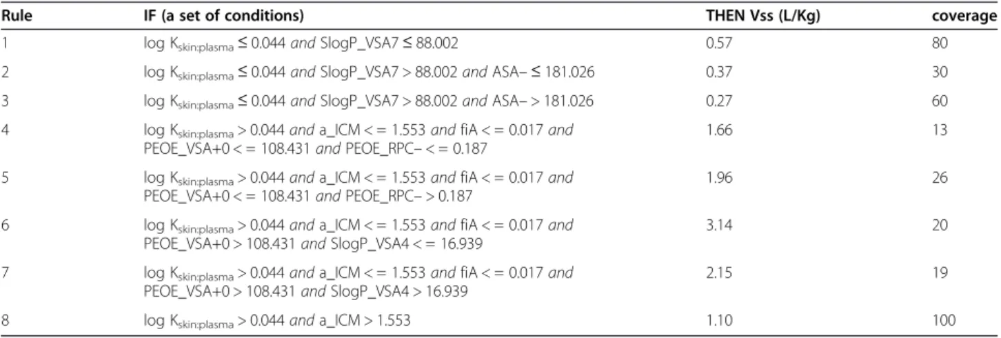
Table 4 shows the subset of rules extracted from the regression tree satisfying the criterion that each rule covers at least 10 compounds in the model selection dataset–where the coverage of a rule is the number of compounds satisfying the conditions in the antecedent of the rule. We focus on these rules because they can be considered more reliable, since the rules covering less than 10 compounds have less statistical support for their predicted log Vss value. Note that, although the regres-sion tree predicts log Vss, rather than Vss, in order to fa-cilitate the interpretation of the results the second column of Table 4 shows the actual Vss value in L/Kg.
Note that log Kskin:plasma occurs in all rules shown in
Table 4 because it is the root node in the regression tree from which the rules were extracted, as mentioned earlier. The first three rules in the table are the only rules in the original tree containing the condition log Kskin:plasma≤0.044, and all those rules predict small Vss
values, considerably below 1 L/Kg. These are the only rules predicting Vss < 1 L/Kg out of the entire set of 18 rules corresponding to the 18 leaf nodes in the ori-ginal tree, i.e., all rules containing the condition log Kskin:plasma> 0.044 predict Vss values higher than 1. The
drugs are known to have low Vss values in general [3,41]. Furthermore, it can be seen from Table 4 that out of these acidic and aromatic compounds, those with large surface area of negatively partially charged atoms (ASA-) have even lower Vss values. Large ASA- indicates compounds with many electronegative atoms, a param-eter similar to polar surface area that is known to have a negative effect in membrane penetration [42,43].
Turning to the rules with log Kskin:plasma> 0.044 in Table 4,
the first four ones (i.e. rules 4–7) are somewhat more diffi-cult to be interpreted, since they have five conditions in their antecedent, but they all have three conditions in common in their antecedents: “log Kskin:plasma> 0.044 and
a_ICM < = 1.553andfiA < = 0.017”, where a_ICM is atom information content and more precisely the entropy of the element distribution in the molecule, and fiA is the fraction of molecules that are ionized as acid at physiologic pH. This part of the rule indicates that compounds with high ability to partition into skin that also contain fewer heteroatoms and are not considerably acidic have relatively high Vss values, according to rules 4–7 in Table 4. Given those three conditions, those rules’ predictions depend on the value of PEOE_VSA+0 and another descriptor. PEOE_VSA+0 is sum of van der Waals surface area of atoms that have a close to neutral partial atomic charge (in the range (0.00,0.05) with PEOE charge calculation [44]). For compounds that satisfy the above three conditions on log Kskin:plasma, a_ICM and fiA, broadly speaking the condition
PEOE_VSA+0 < = 108.431 is associated with smaller Vss values than the condition PEOE_VSA+0 > 108.431, as can be seen by comparing the 4th and 5th rules in Table 4 against the 6th and 7th rules. This indicates higher Vss values for molecules containing mostly neutral (or less polar) atoms. In the case of the two rules with PEOE_ VSA+0 < = 108.431, the use of the descriptor PEOE_RPC– in the last condition to refine the rules does not have much
impact on the predicted Vss. However, in the case of the two rules with PEOE_VSA+0 > 108.431, the predicted value is significantly affected by the value of SlogP_VSA4, another SlogP-related descriptor. This is the sum of van der Waals surface area of specific atom types with logP(o/w) contribu-tion in the range (0.1,0.15]. These atoms include aliphatic carbon and hydrogens and carbonyl groups attached to aromatic rings, which are more prevalent in larger mole-cules with many heteroatoms such as paclitaxel, cyclospor-ine and saquinavir. Consistently with the occurrence of SlogP_VSA7 in the first three rules shown in Table 4, a larger value of SlogP_VSA4 (in this case, > 16.939) is asso-ciated with a smaller predicted Vss, namely 2.15, versus 3.14 when SlogP_VSA4 < = 16.939. Finally, the last rule in Table 4 is “If log Kskin:plasma> 0.044 and a_ICM > 1.553
ThenVss = 1.10”. This rule predicts a Vss of 1.10, which is the lowest predicted Vss value among all 15 rules with con-dition log Kskin:plasma> 0.044 found in the original tree. The
compounds with high a_ICM have a higher ratio of differ-ent heteroatoms in the molecule. It is also the most generic rule found in the original tree, with a coverage of 100 com-pounds that includes β-lactam and quinolone antibiotics, antivirals such as guanosine analogues and similar relatively polar compounds.
In summary, according to the regression tree model built by M5P, the most relevant descriptor for predicting log Vss is log Kskin:plasma, where larger values of this
de-scriptor are associated with higher log Vss values. In addition, other (molecular) descriptors can be used to-gether with log Kskin:plasmato improve log Vss prediction.
In particular, larger values of the related descriptors SlogP_VSA7 and SlogP_VSA4 along with heteroatom ra-tio (a_ICM) are associated with smaller predicted Vss values–in the context of the values of other descriptors occurring in the same rule antecedents as those two descriptors.
Table 4If-Thenregression rules with coverage≥10 extracted from the regression tree built by M5P when using as input descriptors both the predicted log Kt:pfor 12 tissues and a large set of molecular descriptors
Rule IF (a set of conditions) THEN Vss (L/Kg) coverage
1 log Kskin:plasma≤0.044andSlogP_VSA7≤88.002 0.57 80
2 log Kskin:plasma≤0.044andSlogP_VSA7 > 88.002andASA–≤181.026 0.37 30
3 log Kskin:plasma≤0.044andSlogP_VSA7 > 88.002andASA–> 181.026 0.27 60
4 log Kskin:plasma> 0.044anda_ICM < = 1.553andfiA < = 0.017and PEOE_VSA+0 < = 108.431andPEOE_RPC–< = 0.187
1.66 13
5 log Kskin:plasma> 0.044anda_ICM < = 1.553andfiA < = 0.017and PEOE_VSA+0 < = 108.431andPEOE_RPC–> 0.187
1.96 26
6 log Kskin:plasma> 0.044anda_ICM < = 1.553andfiA < = 0.017and PEOE_VSA+0 > 108.431andSlogP_VSA4 < = 16.939
3.14 20
7 log Kskin:plasma> 0.044anda_ICM < = 1.553andfiA < = 0.017and PEOE_VSA+0 > 108.431andSlogP_VSA4 > 16.939
2.15 19
Interpreting the model trees for predicting Vss built by bagging M5P from the descriptors selected by CFS The best regression model built by M5P when using as input only the descriptors selected by the genetic search-based CFS method in a preprocessing phase is a Bagging model, consisting of 10 model trees. The inter-pretation of this regression model is complicated be-cause in each model tree, at each leaf (terminal) node, there is a multiple linear regression model. Each such linear regression equation typically has about 30 descrip-tors. In addition, there are in total 244 such linear re-gression equations in the set of 10 model trees, making their interpretation very difficult in practice. Therefore, in terms of interpretability of the Bagging regression model, we focus mainly on identifying the most relevant descriptors occurring in the internal (non-leaf ) nodes of the 10 model trees, rather than on the descriptors occur-ring in the more numerous linear models.
Identifying only the most relevant descriptors occur-ring in the internal nodes of a set of decision trees (pro-duced, e.g., by Bagging or random forests) is actually relatively common in the literature, and it can be per-formed in different ways. One approach consists of com-puting the percentage of the number of times that each descriptor was selected as the split variable in a tree, out of the number of times the descriptor could be selected (i.e., the total number of nodes in all trees), and then re-port the top descriptors ranked according to that per-centage of selection frequency. This approach was used e.g. in ref. [45], where the top 10 descriptors were re-ported. However, this approach implicitly assumes that the occurrence of a descriptor in a tree node has the same importance regardless of the level of that node in the tree. This assumption is far from true, because, broadly speaking, descriptors at shallow (close to the root) nodes are more relevant than descriptors at deep (far from the root) nodes. This is because, when using any decision tree for predicting the log Vss value of new compounds, each compound will be assigned to a single path in the tree from a root to a leaf node, and in gen-eral shallow nodes occur in many more paths than deep nodes. In particular, a descriptor at the root node will be used to classify every new compound, since it occurs in all paths from the root to any leaf node, as mentioned earlier. In contrast, a descriptor that occurs, say, twice in the tree at deep levels (say at the 4th and 5th levels) will be used to classify much fewer compounds, being there-fore considerably less relevant (despite occurring twice in the tree) than the root descriptor.
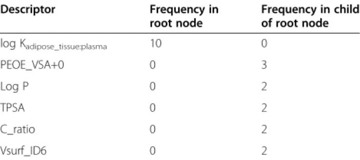
Hence, taking into account that descriptors at shallow tree levels are in general more relevant than descriptors at deep tree levels, we report in Table 5 the descriptors selected by M5P to occur either at the root node or at one of the root’s child nodes, for the best model
produced in our experiments when using as input only the descriptors selected by genetic search-based CFS method applied in a preprocessing step. The table shows only descriptors occurring at least twice as a root or its child in some model tree. We did not consider descrip-tors that were chosen in such roles just once because their occurrence is less reliable and may be due mainly to some stochastic effect of the Bagging method.
In Table 5, it is interesting to note that, in all of the 10 model trees built by Bagging, the descriptor selected for the tree’s root node was log Kadipose_tissue:plasma. Hence,
this can be considered by far the most relevant descrip-tor (out of the descripdescrip-tors pre-selected by the CFS method) as evaluated by the Bagging M5P algorithm. Note that no other tissue’s log Kt:pdescriptor was found
to be very relevant according to the criteria used to pro-duce Table 5. In addition, it should be recalled that log Kadipose_tissue:plasma was selected by the CFS method in a
preprocessing phase, unlike most other tissues’log Kt:ps.
A possible explanation for the much greater importance of log Kadipose_tissue:plasma, by comparison with the other
tissues’log Kt:ps, is that the other tissues’log Kt:pvalues
are redundant with respect to other molecular descrip-tors selected by Bagging; whilst log Kadipose_tissue:plasmais
not only strongly correlated with Vss, but is also non-redundant (or at least less non-redundant) with respect to the other molecular descriptors selected by Bagging. In-deed, it has been reported in the literature that adipose tissue has some special characteristics that may make it particularly distinguishable from other tissues, in the context of Vss prediction. More precisely, adipose tissue is fatty and has a higher percentage of neutral lipids, and in adipose tissue the distribution may be dominated by lipophilicity and hydrophobic interactions, rather than by electronic interactions like in other tissues [39]. In addition, in a recent study proposing a physiologically-based pharmacokinetic model for improving the predic-tion of tissue distribupredic-tion and volume distribupredic-tion of highly lipophilic compounds [19], the simulation of the partition coefficient for adipose tissue was considered Table 5 Most relevant descriptors occurring in the set of 10 model trees produced by Bagging M5P to predict log Vss when using as input only the descriptors selected by genetic search-based CFS
Descriptor Frequency in
root node
Frequency in child of root node
log Kadipose_tissue:plasma 10 0
PEOE_VSA+0 0 3
Log P 0 2
TPSA 0 2
C_ratio 0 2
more sensitive to lipophilicity, by comparison with a non-adipose tissue. Interestingly, another tissue with a more lipophilic composition is skin [39], and, in the re-gression tree built by M5P when using as input the 12 predicted log Kt:p descriptors for different tissues, the
most relevant descriptor chosen for the root node was log Kskin:plasma, as discussed in the previous section.
The next descriptor mentioned in Table 5 is PEOE_VSA+0 (sum of van der Waals surface area of the least polar atoms with low partial atomic charges), which occurred at a child of the root node in 3 out of the 10 model trees.
Another group of relevant descriptors reported in Table 5 includes log P (the log of n-octanol-water parti-tion coefficient), TPSA (Topological Polar Surface Area), C_ratio (the ratio of the number of carbon atoms over the total number of atoms in the compound) and Vsur-f_ID6 (Hydrophobic integy moment), each occurring twice as a child of the root node in the set of model trees. Out of those, log P is a very common measure of lipophilicity, but C_ratio can also indicate compounds’ lipophilicities, since higher carbon ratios indicate fewer polar heteroatoms. Log P and other lipophilicity descrip-tors are often considered relevant predicdescrip-tors of Vss in the literature, since in general increased values of log P lead to increased values of Vss [4,13,14,45]; although this general tendency may not be always true for compounds with extremely high log P values [19]. Also, log P and other lipophilicity descriptors are not identified as rele-vant in every study; an example exception is reported in [22], where the authors did not find any direct relation-ship between Vss and lipophilicity descriptors. However, in that study polarity descriptors often occurred in the Vss models, and the authors noted that polarity is in-versely related to lipophilicity. In a recent study by Paixao et al., who incorporated eight input molecular descriptors in their artificial neural network model based on the literature studies on drug distribution, the relative importance of the descriptors was investigated by varying each input at a time and considering all the other descriptors as constant. This study identified similar parameters, including log P, TPSA and hydro-philicity index as the important determinants of drug distribution [46]. In our experiments, log P seems both to be a relevant descriptor of Vss and to have a positive correlation with Vss.
Discussion
Related work on building QSPkR models for predicting Vss using Obach et al.’s dataset
A direct comparison between the models produced in this work and other models predicting Vss reported in the literature is complicated by the differences in the datasets and types of regression methods used. Concern-ing dataset variations, there are several other studies
based on Obach et al.’s dataset [14], including [5,22,35,45]. However, unlike our work, most of those studies tend to use a substantially smaller version of Obach et al.’s dataset, focusing on a single type of compounds or removing com-pounds that are more difficult to predict for some reason. In particular, the dataset used by Louis and Agrawal [5] contains drugs that belong to the category of anti-infective (J) and sub-categories antibacterial (J01), antimycotics (J02) antimycobacterial (J04) and antiviral (J05) according to the anatomical therapeutic classification (ATC). That dataset contains only 126 compounds, whose Vss varies from 0.05 to 33 L/Kg. The smaller diversity of compounds and their smaller Vss range helps to improve the predict-ive accuracy of the models, at the expense of a more nar-row applicability domain [22,45].
Another study using just a relatively small subset of compounds from Obach et al.’s dataset is reported by Zhivkova and Doytchinova [22]. In that work the dataset consisted of a more heterogenous set of structurally di-verse drugs, but the data used to build the models con-tained only 132 acidic drugs, with an external set containing only 10 acidic drugs that were compiled from ref. [47] and were not included in Obach et al.’s dataset. It is known that acidic drugs tend to have relatively small values of Vss, compared with basic drugs, due to the fact that acids tend to have extensive binding to plasma proteins [41]. Indeed, in the dataset used by Zhivkova and Doytchinova, the compounds’ Vss values range from 0.04 to 15 L/kg, an even smaller range than the one in the dataset used by Louis and Agrawal [5]. Again, the smaller Vss range in the dataset used by Zhivkova and Doytchinova helps to improve the predict-ive accuracy of the models, at the expense of the models’ applicability being restricted to acidic drugs.
In the work of Demir-Kavuk et al. [35], in order to avoid missing values for some descriptors, many com-pounds for which some descriptors could not be calcu-lated were removed from the original Obach et al.’s dataset. More precisely, compounds containing phos-phorous, boron and metal atoms, all macrocycles, and some fragment-like compounds (like Metformin) were removed, which reduced the size of the dataset to 584 compounds. By contrast, in this current work we did not remove any compounds due to missing descriptor values, since the regression methods in the WEKA data mining tool used in this work can cope with missing values (see ref. [24] for details); and this allowed us to work with a somewhat larger dataset of 604 compounds (the size of our Vss-target dataset after the removal of compounds that occurred in our Kt:p-target dataset).
Kt:p-target dataset (they do not use any dataset
equiva-lent to that). In that study idadronic, pamodronic, rise-dronic and zolerise-dronic bisphosphonates were removed from the original dataset based on the argument that these compounds are sequestered to the bones, which hinders their detection in plasma and leads to underesti-mated Vss values. In addition, two antimalarial drugs, namely hydroxychloroquine and chloroquine, were also removed from the original dataset due to their very high Vss values of 700 L/Kg and 140 L/Kg, respectively, which are far from the range of Vss values of the other com-pounds in their dataset (from 0.035 to 60 L/Kg). The lat-ter two drugs were included in our exlat-ternal set, which contributed to a larger prediction error – this issue is further discussed later, when we mention some outliers to our models’prediction.
Related work on decision tree-based regression methods for predicting Vss
Among the several aforementioned studies building QSPkR models from subsets of the Obach et al.’s dataset, the one using the most related data mining method is the work by del Amo et al. [45], where decision trees are used for predicting Vss. By contrast, the studies performed by Demir-Kavuk et al. [35], Louis and Agrawal [5], and Zhivkova and Doytchinova [22] focused mainly on using variations of multiple linear regression, without building decision tree models. Hence, in the following we initially focus on discussing the decision tree-based regression methods used by del Amo et al. [45], contrasting them with the decision tree-based methods used in this work. Next, we discuss other related work on using decision tree-based regression models for predicting Vss.
First of all, note that in del Amo et al.’s work the deci-sion trees are used to predict discrete classes of Vss value, namely classification into ‘high’, ‘medium’ or ‘low’ Vss groups. In contrast, in our work the decision trees perform regression, predicting the numerical value of log Vss.
Another work using decision tree-based methods to predict Vss is reported by Lombardo et al. [13]. The main type of QSPkR model discussed in that study was a hybrid mixture discriminant analysis (MDA)/random forest model. The MDA model is built to discriminate between high or low Vss values, which are defined as above or below the threshold of 10 L/Kg. In addition, two different random forest models are built for predict-ing the numerical values of high and low Vss com-pounds. The prediction of Vss for a new compound is then performed in two stages. Firstly, the MDA model predicts just whether a compound has a high or low Vss. Secondly, the numerical value of Vss is predicted by the corresponding random forest model.
The random forest method used in that study is broadly similar to the bagging method used in our study,
in the sense that both build a model with a set of deci-sion trees. However, each of the two random forests used by Lombardo et al. [13] had 500 trees, making the model more robust but also much slower to build and harder to be interpreted, by comparison with the smaller set of 10 trees in our Bagging model. In addition, the de-cision trees used in the random forest in Lombardo et al.’s work are regression trees, whilst in our work we used instead model trees, which had somewhat better predictive accuracy in our preliminary experiments. Concerning the threshold of 10 L/Kg used to define high and low Vss values for the MDA algorithm, this thresh-old choice seems very ad-hoc. However, to mitigate this problem and try to improve the prediction of Vss for compounds with Vss near the boundary of 10 L/Kg, the random forest predicting high Vss was built using train-ing compounds with Vss≥5 L/Kg, whilst the random forest predicting low Vss was built using as training set all available training compounds. Another difference with respect with our work is that we used only values of Vss in steady state for 604 compounds obtained from Obach et al.’s work [14], whilst in Lombardo et al.’s work [13] the dataset used was not only much smaller, with 384 compounds, but the Vss values for about 10% of compounds was the Vss during the terminal elimination phase, rather than in steady state. These dataset limita-tions are due to the fact that the study by Lombardo et al. predates the availability of the larger dataset of compounds with Vss in steady state made available by Obach et al..
The random forest method was also used by Berellini et al. [47], using a larger set of 669 compounds and using Vss in steady state available from Obach et al.’s work [14]. That study also built a random forest with 500 trees, with the aforementioned pro and cons.
Note that none of those two studies [13,47] reported a systematic interpretation of their random forest models (presumably due to the complexity of interpreting 500 trees); unlike this work, where the trees in a Bagging model were interpreted as discussed earlier.
Outliers of Vss predictions
Discussion section. For example, out of 15 compounds with highest Vss values in the external dataset (11–700 L/Kg), 12 have been underpredicted with a GMFE > 4 by all the three models. This phenomenon of under-prediction of high Vss values was also observed, e.g., in Lombardo et al.’s work [13].
Two outlier compounds whose Vss were substantially under-predicted by our models are hydroxychloroquine and chloroquine, which are antimalarial drugs. These drugs have the very high Vss values of 700 L/Kg and 140 L/Kg, respectively, which are much higher than the highest Vss of compounds in the training set used to build our models. Hence, it is not surprising they are underpredicted by our models. Actually, these two drugs were removed from the dataset used by del Amo et al. [45], which avoided their negative influence in the meas-ure of predictive accuracy of the models in that work, but we preferred not to remove any compound from the dataset based on its prediction difficulty. An explanation for the very high Vss of chloroquine is that it accumu-lates in lysosomes due to an ion-trapping mechanism [48,49]. Another outlier whose Vss was substantially under-predicted in our models is artesunate. Although the Vss of artesunate is 15 L/Kg, its median Vss value obtained for a group of 11 patients with malaria varied from 2.2 to 39 L/Kg [22].
In general, possible explanations for other underpre-dicted outliers in our models could be that they undergo active transport (by influx or efflux transporters) or ex-hibit specific binding to some tissues, or they are stored
in subcellular compartments in specific tissues. For ex-ample, ion-trapping is a mechanism driven by pH gradi-ents that leads to weakly basic drugs accumulation in lysosomes or other acidic membrane-bound intracellular compartments [50]. In addition, some lipophilic weakly basic drugs induce “phospholipidosis”, a phenomenon characterized by histological changes in certain body tissues as a result of the formation of many phospholipid-and cholesterol-rich multivesicular bodies phospholipid-and multilamel-lar bodies that accumulate multilamel-large quantities of the drug and phospholipids [48,51]. However, as pointed out by del Amo et al. [45], it is difficult to know if active transport and specific binding occur to an extent that is large enough to significantly hinder the prediction of Vss, and a precise explanation of outliers would require extensive experimental work, which is out of the scope of this paper.
Conclusions
In this work we have used mainly decision tree-based re-gression methods, but also a feature selection method (correlation-based feature selection with genetic search), to build regression models that predict the Vss of chem-ical compounds based on those compounds’ molecular descriptors and predicted tissue:plasma partition coeffi-cients (Kt:p) in rat.
In order to predict Vss, we investigated three ap-proaches: (a) predicting Vss from both the predicted Kt:p
values and molecular descriptors; (b) predicting Vss from the molecular descriptors only; (c) a two-step ap-proach, where we first used the correlation-based feature