Munich Personal RePEc Archive
Are there gains from including monetary
aggregates and stock market indices in
the monetary policy reaction function?
A simulation study of recent U.S.
monetary policy
Mandler, Martin
University of Giessen
2006
Are there gains from including monetary aggregates
and stock market indices in the monetary policy
reaction function?
- a simulation study of recent U.S. Monetary Policy
Martin Mandler
(University of Giessen, Germany)
First version, November 2006
Abstract
We study how the inclusion of growth rates of monetary aggregates or changes in stock market indices
affects the stabilization performance of optimal monetary policy rules when there is uncertainty about
the structure of the economy. With a simulation model of the U.S. economy we show that the
performance of monetary policy rules that include these variables deteriorates much stronger than
that of rules without them if the true economic structure deviates from the one used to derive the
rule. We also investigate whether money growth and changes in stock market indices help explaining
the Fed’s recent monetary policy.
Keywords: optimal monetary policy, monetary policy reaction function, robust monetary policy
JEL Classification: E47, C15, E52
Martin Mandler
University of Giessen
Department of Economics and Business
Licher Str. 62, 35394 Giessen
Germany
phone: +49(0)641–9922173, fax.: +49(0)641–9922179
1
Introduction
For more than a decade there has been a resurgent interest in the theoretical analysis,
estimation and empirical modeling of monetary policy reaction functions. Since most
of the important central banks implement monetary policy by more or less directly
manipulating short-term interest rates theoretical and empirical research on monetary
policy reaction functions has focused on interest rate rules that express the (desired)
value of the central bank’s policy rate as a function of various state variables describing
current, past or future expected conditions of the economy.
Among the empirical literature, numerous studies have fitted simple interest rate rules,
like the famous Taylor rule (Taylor (1993)) and variants thereof, to the observed path
of the central bank’s interest rate instrument (e.g. Clarida, Galí, and Gertler (1998,
2002), Gordon (2005), Judd and Rudebusch (1998)).1
VAR studies (e.g. Christiano,
Eichenbaum, and Evans (1999) and the literature cited therein), although focussing
on monetary policy “shocks”, i.e. the unsystematic part of monetary policy, provide
estimates of richly parameterized reaction functions.
In the theoretical literature the issue of the optimal design of monetary policy rules
has been discussed intensively. Here, two important questions have to be considered:
1) which variables should be included in the reaction function, that is which variables
should the central bank react to, and 2) how should the central bank react to these
variables? Simple Taylor type rules have the policy rate only react to (forecasts of) the
inflation rate and the output gap/the deviation of the unemployment rate from its
nat-ural level. However, it has also been discussed whether the central bank should react
to the exchange rate as well (e.g. Ball (2000) and Leitemo and Söderström (2005)).2
There has also been a discussion whether growth rates of monetary aggregates should
be included in simple monetary policy rules. In the now standard New Keynesian
models there is no special role for monetary aggregates in the conduct of monetary
1
See also the rather critical discussion in Carare and Tchaidze (2005).
2
Taylor type rules that include exchange rates are estimated by Chadha, Sarno, and Valente (2004)
policy. Money just reacts endogenously to the interest rate set by the central bank.3
However, it has also been argued that even in this type of models monetary aggregates
may contain information that is useful for monetary policy making.4
As far as
mon-etary policy practice is concerned monmon-etary aggregates featured prominently in the
monetary policy strategy of the German Bundesbank and are an important element of
the strategy of the European Central Bank (ECB).5
In contrast, the Federal Reserve
System officially abandoned monetary targets in 1993.
Asset prices, particularly stock prices, are a second group of variables for which it has
been intensively discussed whether or not they should be included in the monetary
pol-icy reaction function. One argument in favor of monetary polpol-icy reacting to changes
in stock prices refers to the predictive content of asset prices for future output and
inflation. These studies recommend that monetary policy should not care about asset
prices per se but should respond to changes in asset prices to the extent that these
signal future deviations of unemployment, output and inflation from its targets (e.g.
Bernanke and Gertler (2000, 2001), Gilchrist and Leahy (2002)). Other authors argue
that asset prices should be targeted by monetary policy in their own right because
drastic changes in asset prices – in particular stock market or housing market crashes
– have strong negative effects on output and employment (eg. Cecchetti et. al. (2000),
Bordo and Jeanne (2002)). However, there are also warnings that including stock
mar-ket variables into monetary policy reaction functions might at best be irrelevant for
the overall economic outcome but might do considerable harm in some circumstances
(Bullard and Schaling (2002)).6
3
For an extended discussion, see Nelson (2003).
4
For example, Coenen, Levin, and Wieland (2005) argue that monetary aggregates convey
informa-tion on the mismeasurement of the output gap. Söderström (2005) shows that assigning a monetary
growth target to the central bank makes discretionary monetary policy more inertial and improves
social welfare relative to standard discretionary policy. Empirical models of the monetary policy
reac-tion funcreac-tion including monetary aggregates have been estimated for the Euro Area by Gerdesmeier
and Roffia (2004).
5
In contrast, Bernanke and Mihov (1997) argue that the Bundesbank did, in fact, not react to
deviations of money growth from its target values.
6
Some empirical studies have investigated the effects of the stock market on monetary policy.
Evidence that the Fed reacts to the stock market is presented e.g. in Bjørnland and Leitmo (2005),
The questions which variables should be included in a monetary policy rule and how
the interest rate should be set in response to them are answered analytically in the
literature on optimal monetary policy rules. Optimal monetary policy rules are
re-action functions that minimize a social/central bank loss function (e.g. Ball (1999),
Clarida, Galí, and Gertler (2001), Giannoni and Woodford (2003a,b), Schmitt-Grohe
and Uribe (2004), Svensson (2003)). In models like these the optimal reaction function
is determined by assumptions about the structural relationships within the economy
and by the parameters of the loss function. The central bank reacts to all economic
variables relative to their predictive content with respect to future values of the central
bank’s goal variables.
These theoretically derived optimal policy rules assume that the central bank knows the
structural relationships within the economy. In practice however, central banks have
to rely on estimated models of the monetary transmission mechanism and only have
a rough understanding of the functioning of the economy. This leads to an important
caveat concerning the practical implementation of optimal monetary policy rules: For
many models optimal reaction functions tend to be quite complex and are very
sensi-tive to changes in the structural assumptions of the model. This sensitivity of optimal
policy rules in combination with the fact that the central bank faces uncertainty about
the structure of the economy has led to a number of studies on “robust” monetary
pol-icy rules. A monetary polpol-icy reaction function is robust if its performance as measured
by a loss function is not very sensitive to changes in the structural equations of the
economic model, that is the value of the loss function does not deteriorate dramatically
if the structural equations or coefficients of the model are changed. Typically, reaction
functions considered in these studies are of a “simple” structure, i.e. they contain only
a small number of variables that the central bank reacts to. Examples are modified
versions of the Taylor rule or difference rules that relate the change in the policy rate
to the deviations in unemployment/output and inflation from their target values (e.g.
Orphanides and Williams (2002), Walsh (2003)). The parameters of the reaction
func-tion are chosen to minimize the central bank’s loss funcfunc-tion under the assumpfunc-tion of a
particular structural economic model. Then, the performance of the optimized simple
reaction function under alternative structural models, i.e. structures different from
the one it was optimized for, is studied by simulating the changed structural model
with the unchanged reaction function and comparing the resulting values of the loss
function or the resulting variances of the central bank’s goal variables (e.g. Walsh
(2003)). This exercise captures the inherent uncertainty of monetary policy makers
about the true structure of the economy. While relatively simple monetary policy
re-action functions generally perform worse than complex ones in the model they were
optimized for, many studies have shown their performance to deteriorate less under
different economic structures (e.g. Levin and Williams (1998), Levin, Wieland, and
Williams (1998), Williams (2003)).
From this research arises a third question. Considering the different variables that
might possibly be included in the policy rule how do these variant policy rules compare
in their robustness with respect to changes in the economic structure? In particular,
how is the relative performance of these rules if central assumptions under which they
were derived turn out to be erroneous?
Our task in this paper is to contribute to this discussion in two ways: First, from a
purely descriptive point of view we ask whether the inclusion of monetary aggregates
or stock market variables in an optimal monetary policy reaction function improves its
ability to explain actually observed monetary policy in the U.S. in the recent period.
This is not meant to conclude whether the Fed did or did not use these variables in
its monetary policy deliberations. Nevertheless, the results can tell us whether, for
ex-ample, monetary aggregates help with explaining the Fed’s behavior, perhaps because
these variables are correlated with information the Fed actually uses when deciding
about the target Federal Funds rate.
Second, we study the questions concerning the design of the monetary policy rule
discussed above by comparing the performance of optimal policy rules containing
al-ternative sets of economic variables. In particular, we focus on the performance of
alternative optimal policy rules when the policymaker is uncertain about the true
structural relationships in the economy.
Our starting point is an empirical model suggested by Sack (2000) who shows that
U.S. monetary policy can be approximated fairly well by a policy rule derived from
an optimal control model in which the structure of the economy is assumed to be
unrestricted empirical model of the structural relationships in the economy. Using this
dynamic structure we solve the dynamic programming problem of the central bank and
derive an optimal monetary policy reaction function. In this we follow the literature
on optimal policy rules but impose relatively few restrictions on the economic model.
By including different sets of variables in our model (monetary aggregates or stock
market indices) we can derive alternative monetary policy rules. We compare how the
interest rate generated by the rule in question “fits” the observed time series of the
Federal Funds rate. If the fit of the policy rule improves by adding a specific economic
variable this might indicate that this variable represents information the Fed looked at
in setting the Federal Funds rate.
Then, we study the robustness of the extended policy rules, i.e. the ones including
money growth or stock market indices, under changing assumptions about the
struc-ture of the economy. We compare them to a restricted rule in which the policy rate
does not respond to these variables. Uncertainty about the structure of the economy
is considered in two different ways: 1) we look at relatively small perturbances of the
economic structure from the one the rule was optimized for by allowing for small
ran-dom variations in the structural coefficients of the model, and 2) we drastically alter
the predictive power of monetary aggregates and the stock market index for the other
economic variables by adding or removing zero restrictions from our structural model.
By these experiments we can show if anything and how much might be gained for
stabilization policy by including money growth or stock market variables in the
pol-icy rule. Fair (2005) performs a similar simulation exercise with optimal polpol-icy rules
within an estimated structural multi-country model. However, he does not study the
robustness of different policy rules and does not focus on monetary aggregates or on
the stock market. In addition, our empirical model imposes much fewer restrictions on
the economic structure.
Our results show that the inclusion of monetary aggregates in the policy reaction
function improves its fit. However, the extended policy rules are much more sensitive
with respect to uncertainty about the economy’s structure than the simple rule which
includes neither money growth nor the stock market index.
U.S. economy and derive the optimal monetary policy rules if only additive uncertainty
is present, that is, if the structural coefficients of the economy are known with certainty.
In section 2.2 we estimate the free parameters of the model and compare the different
policy rules with respect to their ability to track the actually observed Federal Funds
rate and the values for the central bank’s loss function they generate. The optimal
reaction functions under additive uncertainty respond much more aggressive to changes
in economic conditions than it is actually observed. In section 3 we therefore use
an approximation technique from Sack (2000) to derive optimal reaction functions
assuming that the central bank faces uncertainty about the parameters in the structural
economic model (section 3.1). As before, we compare the fit of the simple and the
extended rules (section 3.2). We then study their relative stabilization performance in
the presence of random perturbations to the structural economic model. In addition, we
consider modified versions of our models in which we dramatically alter the information
content of monetary aggregates or stock market variables and compare how the various
rules perform under averse conditions (section 3.2). Finally, section 4 concludes.
2
Optimal policy under additive uncertainty
In this section we derive the optimal monetary policy reaction function for the Fed using
a standard linear-quadratic optimal control approach as described in Sack (2000).7
We
assume that the structure of the economy can be described by a linear structural
model that is based on an estimated vector autoregression. The Fed is assumed to set
its policy rate (the Federal Funds rate) according to a linear policy reaction function.
This reaction function is chosen to minimize a quadratic loss function for unemployment
and inflation.
2.1
Deriving the optimal policy rule
Our analysis starts with the estimation of a structural VAR on monthly data
7
Zt = q
i=0
AiZt−i+
q
i=0
biit−1+νZ
t (1)
it = q
i=0
c′
iZt−i+ q
i=1
diit−1+ν
i
t. (2)
Zt is an (n ×1)-vector of non-policy variables, it is the policy variable (the Federal
Funds rate),q is the number of lags in the VAR,νZ
t is a(n×1)-vector of uncorrelated
structural shocks that is also uncorrelated with the structural policy disturbanceνi t. Ai
are(n×n)matrices andbi andci are (n×1)-vectors. Ztcontains the deviation of the
unemployment rate from the natural rate u, the growth rate of industrial production
y, the inflation rateπ, a rate of inflation for commodity pricescand, alternatively, the
annual growth rate of M1, the annual growth rate of M3, or the annual growth rate of
the S&P 500 stock market index.
We estimate the natural rate of unemployment as in Staiger, Stock and Watson (1997)
from a Phillips curve equation as an unobserved component that follows a random
walk. The inflation rate is the annual growth rate of the Consumer Price Index. Our
measure of commodity price inflation is the annual growth rate of the spot price index
of all commodities from the Commodity Research Bureau.8
Equation (2) represents the estimated (actual) policy reaction function. In our
simula-tions we will replace this equation with the optimal policy reaction function while we
will retain (1) as the description of the structural relations within the economy.
In order to derive the optimal policy reaction function we have to transform the
struc-tural model (1) and (2) into a linear-quadratic dynamic programming problem (see
Sack (2000)). We assume that the Fed maximizes a quadratic objective function
−1
2Et
∞
i=1
βi
(πt+i−π
∗
)2+λu(ut+i−u
∗
)2
, (3)
8
In the VAR literature commodity prices are often used to avoid the “price puzzle”, i.e. an
ob-served increase in inflation following a contractionary monetary policy shock. Introducing commodity
prices often alleviates this problem since they control for expected future inflation. For an extensive
discussion of this issue, see Hanson (2004). For our estimated model commodity price inflation does
not reduce the price puzzle in the impulse response functions. We decided to include this variable
with λu as the weight on the Fed’s employment objective relative to its inflation
ob-jective. Since u is defined as the deviation of unemployment from the natural rate we
setu∗
equal to zero, i.e. we assume that the Fed’s unemployment target is equal to the
natural rate of unemployment.
The structural economic relations (1) are written in state space form as
Xt+1 =F·Xt+Hit+J+µt+1. (4)
The coefficients in F,H,J are derived from (1) as will be described shortly. The state
vector Xt contains current and lagged values of the variables in Zt and its structure
will depend on the assumptions made about the Fed’s information set.
The optimal policy reaction function relates the policy instrument it to the vector of
state variables Xt and solves the Bellman equation
V(Xt) = max it
−(Xt−X
∗
)′
G(Xt−X∗
) +βEt[V(Xt+1)]
(5)
subject to (4). The only non-zero elements inGare the diagonal entries corresponding
to contemporaneous unemployment and inflation which are equal to λu and 1
respec-tively. The vectorX∗
consists of the target values for the state vector. Its only non-zero
elements are the contemporaneous values of the unemployment gap and inflation and
are equal to 0and π∗
.
For this linear quadratic dynamic programming problem the value function will be of
the form
V(X) =X′
ΛX+ 2X′
ω+ρ. (6)
The solution for the optimal policy reaction function is
i∗
t =−(H
′ΛH
)−1(H′ΛF
Xt+H
′ΛJ
+H′
ω), (7)
Λ=−G+βF′
ΛF−βF′
ΛH(H′
ΛH)−1H′
ΛF. (8)
The vector ω is given by
ω = I−βF′
I−ΛH(H′
ΛH)−1H
−1
× GX∗
+βF′
Λ I−H(H′
ΛH)−1H′
Λ
J
. (9)
The dynamics of the economy under the optimal policy reaction function are given by
(4) and (7) with (8) and (9) and imply a recursive structure: The monetary policy
instrument it depends on the current state of the economy Xt and both determine
Xt+1, the state of the economy in the next period. The only source of uncertainty are
the shocks in µt+1 which are not observed by the Fed when it sets it. The optimal
policy reaction function (7) is much less restrictive than a Taylor-type rule and allows
the policy rate to react to current and lagged values of all of the non-policy variables
and to the lagged policy rate itself.
In deriving the optimal policy reaction function we treat the structural economic
pa-rameters in (4) as fixed. In particular, we assume them to be invariant with respect
to the policy reaction function. This assumption is vulnerable to the Lucas critique
(Lucas (1976)) because the parameters in (4) are constructed from the reduced form
coefficients of the VAR in (1) and (2) that were estimated under a particular policy
regime. However, as explained in Sack (2000), the optimal policy rule turns out to be
sufficiently close to the observed policy so that much of the impact of the Lucas
cri-tique is alleviated. In addition, Rudebusch (2005) shows that for empirically reasonable
policy shifts the reduced form coefficients of VARs are largely unaffected.
Since the monetary policy maker observes Xt when setting his policy instrument the
variables to be included in Zt depend on the assumptions about the central bank’s
information set. Sack (2000) assumes that the Fed observes and reacts to the
contem-poraneous values of all variables inZt so thatXtcontains current and lagged values of
Xt = {ut, ut−1,· · · , ut−q, yt, yt−1,· · · , yt−q, πt, πt−1,· · · , πt−q,
ct, ct−1,· · · , ct−q, it−1,· · ·, it−q}. (10)
This assumption implies a recursive structure of the VAR in (1) and (2) in which it is
ordered last, i.e. the variables in Zt do not contemporaneously react to it and b0 = 0.
In this caseF,HandJcan be constructed from the estimated reduced form coefficients
of the VAR. Note that under this assumption it is not necessary to impose additional
identifying assumptions on A0, the matrix of contemporaneous coefficients, in order
to retrieve F,H and J, that is the ordering of the variables in Zt is irrelevant for the
coefficients in (4).9
However, as our goal is to include additional financial markets variables in the system
(4) that are likely to respond contemporaneously to monetary policy actions we also
propose a version of (4) and (10) that puts one variable fromZt (the financial markets
variable)after the policy rate. This assumes that monetary policy does not
contempo-raneously react to the financial markets variable whereas the financial markets variable
is contemporaneously affected by the policy rate. Hence, the current value of the
finan-cial markets variablest =m1t, m3t, sp500t is not part of the central bank’s information
set and the state vector is given by
Xt = {ut, ut−1,· · · , ut−q, yt, yt−1,· · · , yt−q, πt, πt−1q,· · · , πt−q,
ct, ct−1,· · · , ct−q, it−1,· · ·, it−q, st−1,· · · , st−q}. (11)
The construction of (4) for this case is a bit more complicated. The variables ordered
in front ofi in Xt+1 are affected by st but st does not appear in Xt on the right-hand
side in (4) as it is not a state variable monetary policy can react to. We rewrite (4) as
9
As explained in Christiano, Eichenbaum, and Evans (1999) the behaviour of the VAR in response
to a monetary policy shock νi
is independent of the ordering of the variables in front of the policy
rate. However, the exact VAR ordering becomes relevant if we want to simulate the dynamic effects
of the structural shocks inνZ
Φ0Xt+1 =Φ1Xt+Θit+Ψ+ξt+1. (12)
The matrices Φ0 and Φ1 and the vectors Θand Ψcan be constructed from the VAR
estimates. However, while the coefficients in the rows in front of the policy variable
still contain the reduced form coefficients we use the coefficients from astructural
iden-tification for the variables ordered after the policy rate. The structural coefficients are
obtained assuming the recursive ordering(u, y, π, c, i, s).10
The coefficients inΦ0
repre-sent the contemporaneous reactions ofu, y, π andcto each other and their dependence
on the lagged value of s. Note that the structural coefficients of the policy reaction
function (2) are not used for the construction of (4) since the reaction function will
be replaced by (7). The corresponding system (4) is then obtained by premultiplying
with (Φ0)−1
. This will have an effect on the shock vector µt+1. Since ξt+1 in (12) is
equal to
{νu,tZ+1,0,· · · , ν Z
u,t−q+1, ν Z
y,t+1,0,· · · , ν Z
y,t−q+1, ν Z
π,t+1,0,· · · , ν Z π,t−q+1,
νc,tZ+1,0,· · · , νc,tZ−q+1,0,· · · , ν Z
s,t,0,· · · , ν Z
s,t−q} (13)
premultiplying with(Φ0)−1
results inµt+1 being linear combinations of the period-t+ 1
structural shocks to u, y, π, c and the period-t structural shock to s. However, since
µt+1 remains serially uncorrelated and the period-t shock to the financial variable is
not known by the central bank the optimal policy rule remains to be given by (7) with
(8) and (9).
2.2
Estimation and Results
We obtain our structural model from a VAR estimated on monthly data from 1992:1 to
2005:3. A stability test as proposed in Sims (1980) indicates stability of the estimated
VAR coefficients over this period. The VAR is estimated with 12 lags which yields the
10
Using the structural coefficients for all variables leads to the same result for (4) after premultiplying
best fit of the optimal to the actual Federal Funds rate.11
The policy rule (7) contains three free parameters: the discount factor β, the relative
weight of unemployment in the central bank’s loss functionλu, and the inflation target
π∗
. As in Sack (2000) we impose β = 0.996 and estimate λu and π
∗
by minimizing the
sum of squared deviations of the optimal from the actually observed Federal Funds rate.
Thus, we impose the identifying assumption that the Fed’s policy can be adequately
described by our dynamic optimization model (3)-(9).12
For any values of λu and π∗
we compute the optimal Federal Funds rate using the optimal policy reaction function
(7) and the observed values for the state variables inXt. We choose values for λu and
π∗
such as to minimize the sum of squared deviations of the optimal from the observed
Federal Funds rate.13
This estimation procedure yields values λu = 0.15and π∗ = 2.5
for the five variable system (u, y, π, c, i). The estimated weight on unemployment is
considerably lower than in Sack (2000) who finds a value of 0.79 for the period
1984:1-1998:6.14
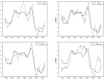
Figure 1 shows the observed path of the Federal Funds rate together with the optimal
Funds rate for various model specifications. The top left panel shows the optimal
Federal Funds rate for the benchmark model with u, y, π, c, i. The optimal policy rule
broadly tracks the actual path of the Funds rate but leads to a much lower interest
rate in the early 90s and a much higher interest rate in 1997 and 1998. It captures the
strong decline of the Funds rate in 2001 but the interest rate starts to increase again
early in 2003. As shown in Table 1 the optimal Funds rate is more than 2.5 times as
volatile as the actual Funds rate.
The other three panels show the optimal Funds rate path for different structural models
11
Sack (2000) uses eight lags. Formal lag-length selection criteria suggest a much lower lag order.
With such a low number of lags the optimal policy rate becomes very volatile and the fit deteriorates
considerably.
12
Matching an optimal monetary policy rule to the historical Fed policy is also done in Rudebusch
(2001) with considerable success.
13
This search procedure is necessary because the matrixΛin (8) cannot be solved for explicitly. As
a consequence we cannot provide information on the precision of the estimates.
14
However, very low weights on output or employment targets in the Fed’s loss function also have
been found in some other studies, e.g. Favero and Rovelli (2003) who find a weight of 0.00125 on the
output gap for the period 1980:3-1998:3. Furthermore,λuturned out to be very sensitive with respect
percent
1992 1994 1996 1998 2000 2002 2004 0 1 2 3 4 5 6 7 8 actual optimal percent
1992 1994 1996 1998 2000 2002 2004 0 1 2 3 4 5 6 7 8 9 actual optimal (m1) percent
1992 1994 1996 1998 2000 2002 2004 0 1 2 3 4 5 6 7 8 9 actual optimal (m3) percent
[image:15.595.78.446.79.356.2]1992 1994 1996 1998 2000 2002 2004 0 1 2 3 4 5 6 7 8 actual optimal (sp500)
Figure 1: Actual and optimal Federal Funds rate for various model
specifi-cations (fixed preference parameters)
(4) holding the parameters λu and π∗ constant. Including the growth rate of M1
(bottom left panel) moves the optimal Funds rate closer to the actual Funds rate in
the mid-90s but produces a stronger interest rate hike in 2000. In addition, the fit at
the beginning and at the end of the sample is worse. Table 1 shows that the overall fit
of the optimal policy rule deteriorates slightly after the inclusion of M1 and that the
optimal Funds rate becomes more volatile relative to the benchmark model.
Including the growth rate ofM3leads to similar results as shown in the top right panel
in Figure 1. Here, the fit of the optimal policy reaction function worsens considerably
and the volatility of the optimal Federal Funds rate increases to 0.64 (see Table 1).
Finally, augmenting our basic model with the growth rate of the S&P500 Index leads
to an even worse fit. Note however, that while the other three specifications have
the optimal Funds rate lagging the steep decline in the actual Funds rate in 2001
the optimal Funds rate for the model with the stock market index leads the observed
Funds rate over this episode. Predicting the expansionary monetary policy of the Fed
variables parameter values SSD σ∆i
u, y, π, c, i λu = 0.15, π∗ = 2.5 158.47 0.4803
u, y, π, c, i, m1 λu = 0.15, π
∗
= 2.5 164.46 0.5590
u, y, π, c, i, m3 λu = 0.15, π∗ = 2.5 203.50 0.6364
u, y, π, c, i, sp500 λu = 0.15, π∗ = 2.5 383.69 0.4694
u, y, π, c, i, m1 λu = 0.20, π∗ = 1.55 85.76 0.5132
u, y, π, c, i, m3 λu = 0.20, π∗ = 1.40 104.78 0.5910
u, y, π, c, i, sp500 λu = 0.475, π
∗
= 2.45 360.91 0.4044
SSD: Sum of squared deviations of optimal from observed Fed-eral Funds rate. σ∆i: Standard deviation of change in optimal
Federal Funds rate (standard deviation of change in observed Federal Funds rate is 0.1821). The optimal Federal Funds rate is calculated using (7) and the actual values of the variables in
Xt.
Table 1: Optimal Federal Funds rate under additive uncertainty - fit and volatility
Table 1 shows the fit of the various model specifications. In the upper panel we imposed
the estimated preference parameters of our benchmark model on all model variants. In
the lower panel we re-estimatedλu andπ
∗
for each model separately. Figure 2 presents
the resulting paths for the optimal policy rate.
The estimation results for the models with M1 and M3 are similar. Both models
produce a small increase in λu and a decline in the inflation target value π
∗
. In both
cases the fit of the policy reaction function improves considerably and far surpasses
that of the benchmark model. The volatility of the policy rate declines but is still
higher than that of the benchmark specification. Figure 2 shows that the behavior
of the optimal Funds rate remains very similar to that shown in Figure 1. For the
model including the S&P500 Index we find only a relatively small improvement in the
fit compared to the upper panel in Table 1 and the sum of squared deviations is still
more than twice as high as that of the benchmark specification. However, the table
shows a drastic change in the estimated weight on the unemployment deviation. Since
only the fit of the reaction functions that include money growth improves relative to
the standard specification, our results so far suggest that monetary aggregates help in
explaining the evolution of the Federal Funds rate over the sample period while the
stock market index does not.
percent
1992 1994 1996 1998 2000 2002 2004 0 1 2 3 4 5 6 7 8 actual optimal percent
1992 1994 1996 1998 2000 2002 2004 0 1 2 3 4 5 6 7 8 actual optimal (m1) percent
1992 1994 1996 1998 2000 2002 2004 0 1 2 3 4 5 6 7 8 actual optimal (m3) percent
[image:17.595.82.445.78.356.2]1992 1994 1996 1998 2000 2002 2004 0 1 2 3 4 5 6 7 8 actual optimal (sp500)
Figure 2: Actual and optimal Federal Funds rate for various model specifi-cations (re-estimated preference parameters)
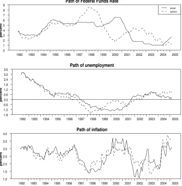
natural rate) and inflation that result from the optimal policy reaction functions. (For
comparison the observed paths of these variables are plotted as well.) The paths are
derived by simulating (4) together with the optimal policy reaction function and using
the same series for the non-policy shocks as historically observed.15
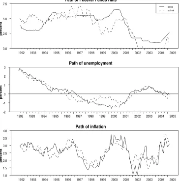
Figure 3 shows
that in the benchmark model the policy rate increases strongly in the mid-90s, comes
down again in the late 90s and runs through a new cycle up to 2005. It is evident that
unemployment and inflation are better stabilized around their respective target values
compared to their actually observed paths.
The optimal policy path for the m1-model starts out with a higher policy rate that
exhibits high volatility for the mid-90s. The Federal Funds rate declines in 1998/99
and rises again in 2000. In 2001 it falls strongly, lagging the observed funds rate, and
15
The starting values for the state vectorXtare the observed values of the variables at the beginning
of the sample period. The shock series are constructed from the reduced form shocks of the VAR for the variablesu, y, π, c and the structural shocks for susing the transformation (12). While Figures 1-2 set the value of Xt in each period to its actually observed value the experiment in Figures 3-6
Path of Federal Funds Rate
percent
1992 1993 1994 1995 1996 1997 1998 1999 2000 2001 2002 2003 2004 2005 0.0
2.5 5.0 7.5 10.0
actual optimal
Path of unemployment
percent
1992 1993 1994 1995 1996 1997 1998 1999 2000 2001 2002 2003 2004 2005 -2
-1 0 1 2 3
Path of inflation
percent
1992 1993 1994 1995 1996 1997 1998 1999 2000 2001 2002 2003 2004 2005 1.0
[image:18.595.77.445.215.590.2]1.5 2.0 2.5 3.0 3.5 4.0
Path of Federal Funds Rate
percent
1992 1993 1994 1995 1996 1997 1998 1999 2000 2001 2002 2003 2004 2005 0.0
2.5 5.0 7.5
actual optimal
Path of unemployment
percent
1992 1993 1994 1995 1996 1997 1998 1999 2000 2001 2002 2003 2004 2005 -2
-1 0 1 2 3
Path of inflation
percent
1992 1993 1994 1995 1996 1997 1998 1999 2000 2001 2002 2003 2004 2005 1.0
[image:19.595.79.445.217.589.2]1.5 2.0 2.5 3.0 3.5 4.0
Path of Federal Funds Rate
percent
1992 1993 1994 1995 1996 1997 1998 1999 2000 2001 2002 2003 2004 2005 0.0
2.5 5.0 7.5
actual optimal
Path of unemployment
percent
1992 1993 1994 1995 1996 1997 1998 1999 2000 2001 2002 2003 2004 2005 -2
-1 0 1 2 3
Path of inflation
percent
1992 1993 1994 1995 1996 1997 1998 1999 2000 2001 2002 2003 2004 2005 1.0
[image:20.595.76.446.89.466.2]1.5 2.0 2.5 3.0 3.5 4.0
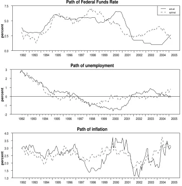
Figure 5: Actual and optimal policy under additive uncertainty - extended model (m3)
hits the zero bound.16
The unemployment and inflation paths seem to be somewhat
smoother but the stabilization gains appear to be limited.
The optimal path for the Funds rate in the m3-model looks broadly similar to the
one in the benchmark model. The the interest rate hike in the mid-to-late 90s is less
pronounced and the Federal Funds Rate declines more slowly beginning in the late
1990s. Similar to the benchmark case inflation and unemployment deviations from
their target values are much lower than for the observed policy.
In the final model the optimal Funds rate tracks the observed Funds rate up to the
mid-16
Path of Federal Funds Rate
percent
1992 1993 1994 1995 1996 1997 1998 1999 2000 2001 2002 2003 2004 2005 0.0
2.5 5.0 7.5
actual optimal
Path of unemployment
percent
1992 1993 1994 1995 1996 1997 1998 1999 2000 2001 2002 2003 2004 2005 -2
-1 0 1 2 3
Path of inflation
percent
1992 1993 1994 1995 1996 1997 1998 1999 2000 2001 2002 2003 2004 2005 1.0
[image:21.595.76.447.210.589.2]1.5 2.0 2.5 3.0 3.5 4.0
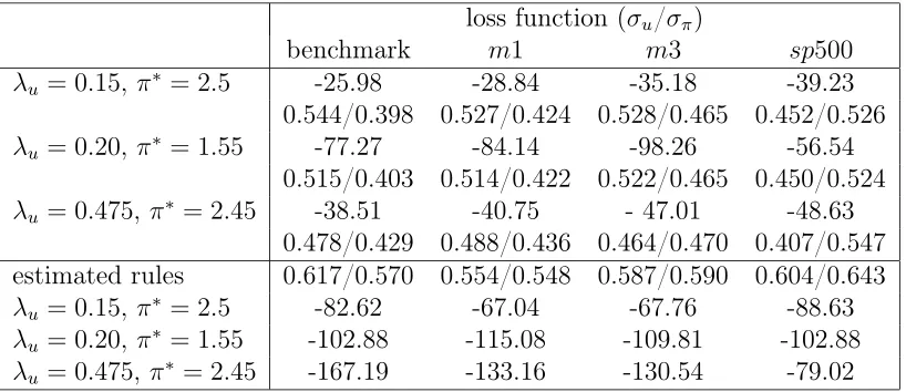
loss function (σu/σπ)
benchmark m1 m3 sp500
λu = 0.15,π
∗
= 2.5 -25.98 -28.84 -35.18 -39.23
0.544/0.398 0.527/0.424 0.528/0.465 0.452/0.526
λu = 0.20,π∗ = 1.55 -77.27 -84.14 -98.26 -56.54
0.515/0.403 0.514/0.422 0.522/0.465 0.450/0.524
λu = 0.475, π∗ = 2.45 -38.51 -40.75 - 47.01 -48.63
0.478/0.429 0.488/0.436 0.464/0.470 0.407/0.547
estimated rules 0.617/0.570 0.554/0.548 0.587/0.590 0.604/0.643
λu = 0.15,π∗ = 2.5 -82.62 -67.04 -67.76 -88.63
λu = 0.20,π
∗
= 1.55 -102.88 -115.08 -109.81 -102.88
λu = 0.475, π∗ = 2.45 -167.19 -133.16 -130.54 -79.02
[image:22.595.80.489.74.251.2]σu, σπ: Standard deviation of unemployment and inflation
Table 2: Performance of different optimal reaction functions under additive uncertainty
90s. It follows a path similar to the one in the benchmark model but less pronounced
and more gradual. The policy rate does not rise in the late 90s as it was historically
the case.
It is obvious that the optimal policy reaction functions prescribe a more aggressive
behavior of the policy rate than actually observed. However, they also imply a strong
persistence of the Federal Funds rate. As already pointed out by Sack (2000), this
persistence is caused by the high degree of serial correlation in the variables the central
bank reacts to.
Table 2 shows the average values of the loss function under the different optimal policy
rules obtained from simulating (4) and (7) and using 500 draws of random shock series
µfor the non-policy variables. Since we found some variation in the estimated
prefer-ence parameters for the different models the table shows the values of the loss function
for these various parameter combinations. Below the values of the loss function are the
average standard deviations of the unemployment gap and the inflation rate obtained
from the 500 simulated time series for inflation and unemployment.
In the first row are the values of the loss function obtained with the parameter
esti-mates from the benchmark model. Including additional variables in the central bank’s
information set and policy reaction function does not improve the loss function. We
get a similar result for the parameter estimates from the model with the stock market
func-tion. Again, the benchmark model performs better than the three extended models.
A different result can be found for the model in the second row which uses the
pa-rameter estimates from the model withM1.17
Here, the benchmark model is superior
to the M1 model which in turn is better than the M3 model but the smallest loss
results for the model including the stock market index. However, the inflation target
π∗
is unreasonably small so that this result should be taken with caution.18
. In the
lower panel we show the values of the loss function that result from using the estimated
policy reaction functions, that is the estimated equation (2) for each model. It is
obvi-ous that the more aggressive optimal reaction functions offer substantial stabilization
gains. This is also evident by looking at the standard deviations of the unemployment
gap and inflation which are always lower for the optimal reaction functions.19
Overall, Table 2 shows that there is not much evidence that including monetary
ag-gregates or stock market variables in the monetary policy reaction function offers
sub-stantial stabilization gains. However, in Table 1 we found some evidence for the ability
of monetary aggregates to contribute to explaining the actually observed behavior of
the Federal Funds rate. A possible explanation for money growth being helpful in
explaining the Funds rate in this model is that in fitting the optimal to the observed
Funds rate our model has to try to mimic its high degree of autocorrelation. Since
both money growth rates exhibit a high degree of persistence themselves, reacting to
these variables strengthens the persistence of the optimal Funds rate and improves the
fit.20
In the next section, we will modify our model by introducing uncertainty about
the structure of the economy. This will make the optimal reaction function respond
less aggressively to changes in economic conditions and introduce a higher degree of
persistence into the optimal Federal Funds rate path. This more persistent behavior
of the optimal Funds rate might be able to explain the observed Funds rate without a
need for monetary aggregates.
17
Since the estimates for the model withM3 only differed slightly forπ∗, we did not consider this
parameter combination on its own.
18
The ECB aims for an inflation rate of 2% or slightly below while the Fed is generally believed to have a higher implied inflation target
19
The price for this enhanced stabilization is an about 2-3 times higher standard deviation of the changes in the Federal Funds rate (not shown) under the optimal reaction functions.
20
3
Optimal policy under parameter uncertainty
In the last section we assumed that the central bank knew the true dynamic structure
of the economy as represented in (4) and that all uncertainty was due to the
stochas-tic disturbances in µ. With a quadratic loss function and linear constraints certainty
equivalence holds, that is additive uncertainty does not affect the optimal policy
reac-tion funcreac-tion. However, in the real world, central banks can only rely on an estimated
model of the structural relations within the economy and this estimated model must
not necessarily be correct. In our study we follow Sack (2000) and focus on uncertainty
about the true values of the coefficients in (4). Brainard (1967) shows that parameter
uncertainty about the effects of policy on the economy can lead to a less aggressive
policy compared to that under certainty equivalence. However, other studies have
con-cluded that parameter uncertainty must not necessarily make monetary policy more
cautious but may actually lead to a more aggressive monetary policy (e.g. Söderström
(2002)).21
3.1
Deriving the optimal policy reaction function
To account for parameter uncertainty Sack (2000) proposes to rewrite (4) as
ˆ
Xt+1 =F·Xˆt+Hit+J+µt+1, (14)
whereXˆt=Et−1Xˆt is the forecast ofXt based on timet−1information. The optimal
policy sets the interest rate as a function of Xˆt. This implies that the central bank
reacts to shocks to the elements of Xt with a lag of one period.
22
Sack (2000) shows that the solution to the optimization problem (5) can be
approxi-mated by the Bellman equation
21
We assume the economic structure to be constant over the sample period and thus take no account of possible structural change. We also do not consider learning models in which the policymaker gradually improves his estimate of the structure of the economy as more and more data become available – possibly gaining additional data by variations in policy – as, for example, in Orphanides and Williams (2005), Sack (1998) and Wieland (1999, 2000).
22
V( ˆXt) = max it
− Xˆt−X
∗
′
G Xˆt−X∗
− Xˆ′
tKXˆt+ 2 ˆXtL
+βEt
V( ˆXt+1)
. (15)
subject to (14). This reformulation of the problem leaves the dynamic structure of
equation (4) unchanged – the coefficients are still given by those derived from the VAR
– and incorporates the effects of parameter uncertainty into the loss function. The
matrix K and the vector L are weighted sums of the variance-covariance matrices of
the parameters describing the dynamic behaviour of the variables in the central bank’s
loss function. K = Σβ(π) +λuΣβ(u), where Σβ(n), n = u, y, is the covariance matrix
between the coefficients within the equation of current unemployment and inflation in
(4) and L is a similar construction containing the covariance of the n-th equation’s
elements inF with the n-th element of the vector J. The solution in (16) is based on
the assumption that K and L are constant.23
One problem with this approach is that Xˆt+1 =F·Xt+Hit+J actually evolves from
Xt and not from Xˆt so that µt+1 in (14) picks up a term related to Xt −Xˆt. µ is
still uncorrelated with Xˆt and the dynamics in (14) remain unbiased. However, the
accumulation of the effects of Xt−Xˆt through time leads to an increasing variance of
µ. Hence, the solution (15) is only an approximation to the solution of the dynamic
programming problem under parameter uncertainty. Sack (2000) shows that the
opti-mal solution can be retrieved by assigning different weights to the first and the second
term in (15), that is by replacingG with Gˆ= (1−ρ)G,K with Kˆ =ρK, and L with
ˆ
L=ρL. ρ is chosen to minimize the loss function.24
23
The values of these matrices are derived from the variance-covariance matrix estimated over the complete sample period. This probably leads to an underestimation of the actual degree of uncertainty the central bank is facing.
24
Specifically, for a given value of ρ we compute from (16) the optimal policy reaction function under parameter uncertainty. We then construct a hypothetical path for the policy rate using the actually observed values ofXtat each point in time and search for the combination ofλu andπ∗that
minimizes the sum of squared deviations of the optimal from the actually observed policy rate. This gives us a set ofρand associated combinationsλu, π∗. For each combinationρ, λu, π∗ we then draw
500 sets of coefficients inF,HandJ, based on the variance-covariance matrix of their VAR estimates
and then simulate (4) with these new coefficients but using the optimal policy rule. Finally, we select forρ, λuandπ∗that combination among the ones available that yields the lowest average value of the
The optimal policy reaction function is similar to that under additive uncertainty with
Xt being replaced byXˆt
i∗
t =−(H
′
ΛH)−1 H′
ΛFXˆt+H′
ΛJ+H′
ω. (16)
The Riccati equation becomes
Λ=−Gˆ −Kˆ +βF′ΛF
−βF′ΛH
(H′ΛH
)−1H′ΛF
, (17)
and
ω = I−βF′ I
−ΛH(H′ΛH
)−1
H
−1
× GˆX∗
−Lˆ+βF′Λ I
−H(H′ΛH
)−1
H′ΛJ
. (18)
3.2
Estimation and Results
As Table 3 shows, the volatility of the optimal policy rate decreases relative to the
situation under additive uncertainty (Table 1). In the upper panel we find the results
for holding the preference parameters fixed at the values from the upper panel of Table
1 and only estimating ρ. The volatility of the optimal Federal Funds rate is much
lower than in Table 1 but is still higher than the actually observed one. The fit of the
optimal policy rule improves strongly
The lower panel shows the results after re-estimating the preference parameters
to-gether with ρ. For the first model the volatility of the optimal policy increases by a
small amount while it declines for the other models. The fit improves strongly for the
standard model and the models withm1and the stock market index but only slightly
for them3-model. The estimated preference parameter λu is lower than in Table 1 for
all specifications and the estimated target value for inflation π∗
falls into a relatively
close range for all models. In terms of fit both models with growth rates of monetary
aggregates turn out to be superior to the benchmark model. These results indicate
variables parameter values SSD σ∆i
u, y, π, c, i λu = 0.15, π∗ = 2.5, ρ= 0.20 92.63 0.4029
u, y, π, c, i, m1 λu = 0.15, π
∗
= 2.5, ρ= 0.20 80.94 0.4890
u, y, π, c, i, m3 λu = 0.15, π∗ = 2.5, ρ= 0.20 59.38 0.4832
u, y, π, c, i, sp500 λu = 0.15, π∗ = 2.5, ρ= 0.20 254.30 0.3896
u, y, π, c, i λu = 0.05, π∗ = 2.60,ρ= 0.30 72.80 0.4111
u, y, π, c, i, m1 λu = 0.05, π∗ = 2.55,ρ= 0.40 46.00 0.4400
u, y, π, c, i, m3 λu = 0.10, π
∗
= 2.40,ρ= 0.20 57.29 0.4776
u, y, π, c, i, sp500 λu = 0.05, π∗ = 2.60,ρ= 0.60 124.17 0.3377
SSD: Sum of squared deviations of optimal from observed Fed-eral Funds rate. σ∆i: Standard deviation of change in optimal
[image:27.595.111.461.75.208.2]Federal Funds rate (standard deviation of change in observed Federal Funds rate is 0.1821). The optimal Federal Funds rate is calculated using (16) and the actual values of the variables inXt.
Table 3: Optimal Federal Funds rate under parameter uncertainty - fit and volatility
of the Federal Funds rate.
Figure 7 shows the optimal paths of the policy rate based on the parameter estimates
in the lower panel of Table 3. As in Figure 1 the time series are those that would
be obtained if the variables in Xt were at their historically observed values at each
point in time. All models do fairly well in capturing the behaviour of the Federal
Funds rate through our sample period. Compared to Figures 1 and 2 the optimal
Funds rate evolves more smoothly. All models mimic the strong interest rate decline in
2001 but suggest an even stronger lowering of the interest rate. The first three models
also capture the interest rate increase in 1999/2000 but the timing is only
approxi-mately correct for the m3-model. Interestingly, the sp500-model suggests a monetary
tightening beginning in 2002 well before the Fed actually began raising interest rates
again in 2004. In contrast to the extended models, the benchmark model prescribes an
additional peak in the Funds rate in 1997/1998 that is much more pronounced than
actually observed.
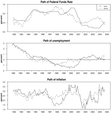
In Figure 8 we present the simulated paths of the policy rate, unemployment (deviation
from natural rate) together with the actually observed path of the respective variables.
percent
1992 1994 1996 1998 2000 2002 2004 0 1 2 3 4 5 6 7 actual optimal percent
1992 1994 1996 1998 2000 2002 2004 0 1 2 3 4 5 6 7 8 actual optimal (m1) percent
1992 1994 1996 1998 2000 2002 2004 0 1 2 3 4 5 6 7 8 actual optimal (m3) percent
[image:28.595.81.446.78.354.2]1992 1994 1996 1998 2000 2002 2004 0 1 2 3 4 5 6 7 actual optimal (sp500)
Figure 7: Actual and optimal Federal Funds rate for various model specifi-cations under parameter uncertainty
the optimal policy reaction function under parameter uncertainty (16) and using the
same series for the non-policy shocks as observed historically.
The path for the optimal policy rate for the standard model u, y, π, c, i looks similar
to that in Figure 3. For all the simulated paths the volatility of the Federal Funds
rate is similar to its actually observed volatility (0.1821) (benchmark model: 0.2502,
m1-model: 0.2618 (not shown), m3-model: 0.2719 (not shown) , sp500-model: 0.1913
(not shown)).
In Table 4 we compare the stabilization performance of the different optimal rules in
the presence of uncertainty about the economy’s structural relationships. Specifically,
we compute the average values of the central bank’s loss function and the standard
deviations of unemployment and inflation for each of the augmented rules and
com-pare them to those of the simple rule. In each comparison one aspect of uncertainty
is captured by combining the policy rule with a structural model (4) that differs from
the originally estimated model by drawing from the distribution of the estimated
Path of Federal Funds Rate
percent
1992 1993 1994 1995 1996 1997 1998 1999 2000 2001 2002 2003 2004 2005 0
1 2 3 4 5 6 7 8 9
actual optimal
Path of unemployment
percent
1992 1993 1994 1995 1996 1997 1998 1999 2000 2001 2002 2003 2004 2005 -1.8
-1.2 -0.6 0.0 0.6 1.2 1.8 2.4 3.0 3.6
Path of inflation
percent
1992 1993 1994 1995 1996 1997 1998 1999 2000 2001 2002 2003 2004 2005 1.0
[image:29.595.79.444.216.589.2]1.5 2.0 2.5 3.0 3.5 4.0
true model loss function (σu/σπ)
preference parameters benchmark m1 m3 sp500
u, y, π, c, i -106.56 -450.39 -544.57 n.a.
λu = 0.05,π
∗
= 2.60, ρ= 0.30 1.29/0.75 1.69/1.25 1.51/1.03 n.a.
u, y, π, c, i, m1 -127.19 -135.44 – –
λu = 0.05,π∗ = 2.60, ρ= 0.30 1.41/0.80 1.36/0.86 – –
u, y, π, c, i, m3 -223.97 – -224.57 –
λu = 0.05,π∗ = 2.60, ρ= 0.30 1.53/1.09 – 1.52/1.03 –
u, y, π, c, i, sp500 -116.98 – – -168.30
λu = 0.05,π
∗
= 2.60, ρ= 0.30 1.41/0.78 – – 1.26/1.00
u, y, π, c, i, m1 -251.97 -141.02 – –
λu = 0.05,π
∗
= 2.55, ρ= 0.40 1.53/1.19 1.40/0.89 – –
u, y, π, c, i, -110.36 -537.83 – –
λu = 0.05,π∗ = 2.55, ρ= 0.40 1.34/0.76 1.75/1.18 – –
u, y, π, c, i, m3 -260.51 – -205.30 –
λu = 0.10,π∗ = 2.40, ρ= 0.20 1.56/1.11 – 1.40/0.99 –
u, y, π, c, i -124.91 – -373.99 –
λu = 0.10,π∗ = 2.40, ρ= 0.20 1.35/0.76 – 1.77/1.10 –
u, y, π, c, i, sp500 -122.61 – – -161.33
λu = 0.05,π∗ = 2.60, ρ= 0.60 1.17/0.65 – – 1.30/0.97
u, y, π, c, i -126.84 – – n.a.
λu = 0.05,π
∗
= 2.60, ρ= 0.60 1.42/0.79 – – n.a.
[image:30.595.79.491.231.556.2]σu, σπ: Standard deviation of unemployment and inflation
with random coefficient draws and for each draw we simulate the model 500 times
using random series for the shocks inµdrawn using the variance-covariance matrix of
the residuals obtained from imposing the drawn coefficients on the model. In addition
we consider a more serious element of uncertainty: We compute values for the loss
function of the augmented rules assuming that the additionally included variable (M1,
M3, or the stock market index) has no predictive power for future values of
unemploy-ment and inflation, that is we assume that the structural assumptions made for the
standard model are in fact the correct ones. In addition to the always applied random
changes to the parameters this implies setting some of the coefficients on the money
or stock market variable in the structural model to zero.25
In turn, we will perform a
similar simulation for the simple rule by assuming that the variables ignored in it (M1,
M3, or the stock market index) in fact help to predict future values of unemployment
and inflation, that is we assume the structural models used to derive the augmented
rules to be correct (up to some small random changes in the parameters) but combine
them with the simple rule. Naturally, the performance of each rule will deteriorate if
it is combined with a structurally different model. The robustness of each rule
there-fore can be evaluated from how much worse each rule performs under these different
circumstances.
The top panel in Table 4 presents the results from using the preference parameter
values originally estimated for the standard system (u, y, π, c, i), that is from the first
row in the second panel of Table 3.26
The first two rows show the average values of
the loss function and the standard deviations of unemployment and inflation for all
rules assuming that monetary aggregates and the stock market index do not help in
forecasting future inflation and unemployment. Naturally, the rule derived from the
standard model performs best while the loss function worsens strongly for the two rules
that include monetary growth rates. If we use the rule with the stock market index
and impose the restrictions that changes in theS&P500 have to predictive content for
the other variables in the system almost all randomly drawn coefficient matrices result
25
We assume thatsreacts to all other variables in the system but that these variables do neither react to current nor lagged values ofs
26
Sinceλu and π∗ are elements of the loss function they have an important direct impact on the
in unstable systems.
The third and fourth rows in the top panel compare the optimal rule for the standard
system to the rule including the growth rate of M1 assuming that M1 helps in
fore-casting the other variables, that is using the structural model which includes M1. The
next two rows perform the same exercise with the standard and the augmented rule for
the system including M3 and the final two rows show the results for the comparison
of the standard to the augmented (sp500) rule assuming that the stock market index
has predictive content. The standard rule always has a lower value of the loss function
both in the standard model (top row) and in the other models. That implies that
even if one of the extended models is assumed to be the correct model the standard
rule is superior to the augmented rules because the latter ones are very vulnerable to
uncertainty about the coefficients of the structural model.
The following panels show the results of analogous exercises using the estimated
prefer-ence parameters from the m1, m3, and sp500 models, respectively. In the m1 and m3
case the standard rule is inferior to the extended rule if the extended model is assumed
to be the correct one. However, the loss function for the m1 augmented rule
deteri-orates much stronger (from -141.02 to -537.83, i.e. by 280%) than the standard rule
(from -110.36 to -251.97, i.e. by 130%) if combined with the “wrong” model. Clearly
for this set of preference parameters the standard rule is more robust than the m1
augmented rule. For the preference parameters estimated from the m3model (next to
last panel in Table 3) the comparison between them3augmented rule and the standard
rule is less clear cut. Here the average loss function value of the m3 augmented rule
increases by 82% (from -205.30 to -373.99) if M3 becomes non-informative while the
average loss under the standard rule increases by 108% if the growth rate of M3 in fact
contains important forecasting information. For these parameter values the m3
aug-mented rule appears to be slightly more robust than the standard rule. In the bottom
panel we impose the preference parameters estimated from the model that includes the
stock market index (last row of Table 3). Here again we encounter the problem that
combining thesp500 augmented rule with a model in which the stock market index has
no predictive power leads to an unstable dynamic system. However, as the standard
rule already dominates the sp500 augmented rule even if we take the extended model
standard model.
To sum up, the results in Table 4 strongly indicate that a rule without monetary
growth rates or a stock market index is more robust than the augmented optimal rules.
If we apply the minimax criterion, that is if we select the policy rule which minimizes
the maximum possible loss, the standard reaction function beats all other contenders
handsomely. In particular, including the stock market index in the information set of
the central bank leads to worse results than the standard rule. Obviously, if we assume
uncertainty about the structural relationships in the economy the stock market index
must introduce a lot of noise into the model. Responding to such a noisy signal leads
to adverse economic results.
4
Conclusion
We have shown that the recent path of the Federal Funds rate can be approximated by
an optimal monetary policy reaction function derived from a relatively simple
struc-tural model. Having the Federal Funds rate also responding optimally to growth rates
of M1 or M3 improved the ability of the optimal rule to explain the actual time series
of the Federal Funds rate. In contrast, including a stock market index did not improve
the fit of the optimal policy rule. These results show that monetary aggregates contain
some information that helps with explaining Fed behavior. This does not imply that
the Fed in fact reacts to changes in the growth rates of monetary aggregates but that
money growth might be correlated with some variables that the Fed looks at in setting
interest rates, for example credit growth, financial market conditions etc. While the
optimal reaction functions reproduce the general path of the Funds rate quite well, the
simulated interest rate is much more volatile than was actually observed.
Taking account of uncertainty about the true economic structure affects the
compar-isons between different optimal policy rules in various ways. It was shown that the
volatility of the optimal Federal Funds rate declined for all the policy rules under
consideration. The policy rules that included monetary growth rates still tracked the
actually observed Funds rate more closely than the policy rule without them.
Federal Funds rate in 2001. Even those rules that do not react to changes in stock
prices recommended a strong decline in the Federal Funds rate as an optimal response.
We then studied the robustness of the different policy rules and showed that the
stabi-lization performance of the simple rule (that did not include monetary growth rates or
a stock market index) worsened less than that of the other optimal rules if the model
under which it was derived is assumed to be wrong. The simple rule is less sensitive to
changes in the structure of the economy or errors in the estimation of the structural
relationships. While money growth or stock market data might have some predictive
power for the other economic variables, the possible gains for stabilization policy from
this, however, are often compensated by the loss in stabilization performance that
re-sults from unstable and noisy relationships between these financial variables and the
rest of the economic system.
Overall, our model shows that assigning a prominent role to monetary aggregates in
the formulation of monetary policy might have some benefits but also carries high
risks. Such a strategy is only attractive if the policymaker has high confidence in his
knowledge of the structural relationships within the economy. The stock market
in-dex, however, has such an unreliable relationship to the other economic variables that
including it consistently in the the policy rule will lead to a severe deterioration of the
References
Ball, Laurence (1999), Efficient Rules for Monetary Policy, International Finance 2, 63-83.
Ball, Laurence (2000), Policy Rules and External Shocks, NBER Working Paper No. 7910.
Bernanke, Ben S. and Mark Gertler (2000), Monetary Policy and Asset Price Volatility, NBER Work-ing Paper No. 7559.
Bernanke, Ben S. and Mark Gertler (2001), Should Central Banks Respond to Movements in Asset Prices?, American Economic Review 91, 53-57.
Bernanke, Ben S. und Ilian Mihov (1997), What Does the Bundesbank Target?, European Economic Review 41, 1025-53.
Bjørnland, Hilde and Kai Laitmo (2005), Identifying the Interdependence between US Monetary Policy and the Stock Market, Working Paper, University of Oslo.
Bordo, Michael D. and Olivier Jeanne (2002), Monetary Policy and Asset Prices: Does ’Benign Neglect’ Make Sense?, International Finance 4, 139-64.
Brainard, William (1967), Uncertainty and the Effectiveness of Policy, American Economic Review Papers and Proceedings 57, 411-25.
Bullard, James B. and Eric Schaling (2002), Why the Fed Should Ignore the Stock Market, Federal Reserve Bank of St. Louis Review 84:2, 35-42.
Carare, Alina and Robert Tchaidze (2005), The Use and Abuse of Taylor Rules: How Precisely Can We Estimate Them?, IMF Working Paper 05/148.
Cecchetti, Stephen G., Hans Genberg, John Lipsky, and Sushil Wadhwani (2000), Asset Prices and Central Bank Policy, International Centre for Monetary and Banking Studies.
Chadha, Jagjit S., Lucio Sarno, and Giorgio Valente (2004), Monetary Policy Rules, Asset Prices, and Exchange Rates, IMF Staff Papers 51, 529-52.
Christiano, Lawrence J., Martin Eichenbaum, and Charles L. Evans (1999), Monetary Policy Shocks: What Have we Learned and to What End?, in: Taylor, John B. and Michael Woodford (1999), Handbook of Macroeconomics, Vol. 1A, Elsevier, 65-148.
Clarida, Richard, Jordi Galí, and Mark Gertler (1998), Monetary Policy Rules in Practice: Some International Evidence, European Economic Review 42, 1033-67.
Clarida, Richard, Jordi Galí, and Mark Gertler (2001), Optimal Monetary Policy in Closed versus Open Economies: An Integrated Approach, NBER Working Paper No. 8604.
Clarida, Richard, Jordi Galí, and Mark Gertler (2002), Monetary Policy Rules and Macroeconomic Stability: Evidence and Some Theory, Quarterly Journal of Economics 115, 147-80.
Coenen, Günter, Andrew Levin, and Volker Wieland (2005), Data Uncertainty and the Role of Money as an Information Variable for Monetary Policy, European Economic Review 49, 975-1006.
D’Amico, Stefania and Mira Farka (2003), The Fed and the Stock Market: An Identification Based on Intraday Futures Data, Working paper, Columbia University.
D’Agostino, Antonello, Luca Sala, and Paolo Surico (2005), The Fed and the Stock Market, Working Paper.