Bulk Viscous Bianchi Type V Space Time with Generalized Chaplygin Gas and with Dynamical G and Λ

http://dx.doi.org/10.4236/ijaa.2015.53025

Bulk Viscous Bianchi Type V Space-Time

with Generalized Chaplygin Gas and with

Dynamical G and

Λ

Shubha S. Kotambkar1, Gyan Prakash Singh2, Rupali R. Kelkar3

1_{Department of Applied Mathematics, Laxminarayan Institute of Technology, Rashtrasant Tukadoji Maharaj}

Nagpur University, Nagpur, India

2_{Department of Mathematics, Visvesvaraya National Institute of Technology, Nagpur, India}

3_{Department of Applied Mathematics, S. B. Jain Institute of Technology, Management and Research,}

Nagpur, India

Email: [email protected], [email protected], [email protected]

Received 16 March 2015; accepted 25 September 2015; published 28 September 2015

Copyright © 2015 by authors and Scientific Research Publishing Inc.

This work is licensed under the Creative Commons Attribution International License (CC BY).

http://creativecommons.org/licenses/by/4.0/

Abstract

In this paper, bulk viscous Bianchi type V cosmological model with generalized Chaplygin gas, dy-namical gravitational and cosmological constants has been investigated. We are assuming the condition on metric potential R R m_n

R R t

₁ ₂

1 2

= = . To obtain deterministic model, we have considered physically plausible relations like P= + Πp , η η ρ= 0 r and the generalized Chaplygin gas is

de-scribed by equation of state p B_α

ρ

−

= . A new set of exact solutions of Einstein’s field equations has been obtained in Eckart theory, truncated theory and full causal theory. Physical behavior of the models has been discussed.

Keywords

Bianchi Type V, Gravitational Constant, Cosmological Constant, Bulk Viscosity, Chaplygin Gas

1. Introduction

isotropic. But it is widely believed that FLRW model does not give a correct matter description in the early stage of universe. The theoretical argument [1] and the recent experimental data support the existence of an aniso-tropic phase, which turns into an isoaniso-tropic one during the evolution of the universe. Anisoaniso-tropic model plays significant role in description of evolution of the early phase of the universe and also helps in finding more gen-eral cosmological models than the isotropic FRW models. This motivates researcher for obtaining exact aniso-tropic solution for Einstein’s field equations as a cosmologically accepted physical models for the universe (in the early stages). The study of Bianchi type V cosmological model being anisotropic generalization of open FRW models is important to study old universe. A number of authors have investigated Bianchi type V cosmo-logical model in general relativity in different context [2]-[15]. Rajbali and Seema Tinkar have discussed Bianc-hi type V bulk viscous Barotropic fluid cosmological model with variable G and Λ. Recently Yadav and Sharma

[16] and Yadav [17] have discussed about transit universe in Bianchi type V space-time with variable G and Λ.

It has been widely discussed in the literature that during the evolution of the universe, bulk viscosity can arise in many circumstances and can lead to an effective mechanism of galaxy formation [18]. It is known that real fluids behave irreversibly and therefore it is important to consider dissipative processes both in cosmology and in astrophysics. To consider more realistic models, one must take in to account the viscosity mechanism. Bulk viscosity leading to an accelerated phase of the universe today has been studied by Fabris et al. [19]. Very re-cently Kotambkar et al. [20] have investigated anisotropic cosmological models with quintessence considering the effect of bulk viscosity.

A wide range of observations strongly suggest that the universe possesses non zero cosmological term [21]. The astronomical observations [22] [23] support that the expansion of the universe is accelerated. It suggests that there exists a new component in universe named as dark energy with negative pressure. A natural explana-tion for the accelerated expansion is due to a positive small cosmological constant. An attenexplana-tion has been paid to cosmological models with non zero cosmological term Λ [21] [24], whose existence is favored by supernovae SNe Ia observations (refer to [22] [23]) which are consistent with the recent anisotropy measurements of the cosmic microwave background (CMB) made by the WAMAP experiment [25]. Sahni and Starobinski [26] have presented detailed discussion on current observational situation focusing on cosmological tests on Λ.

Time varying G has many interesting consequences in astrophysics. Cunuto and Narlikar [27] have shown that G-varying cosmology is consistent with what so ever cosmological observations available at present. A new approach is appealing; it assumes the conservation of the energy momentum tensor which consequently gives G

and Λ as coupled fields similar to the case of G in original Brans-Dicke theory. The cosmological model with variable G and Λ has been investigated by several researchers [28]-[32]. A number of researchers have dis-cussed various anisotropic cosmological models with variable G and Λ [33]-[37].

According to recent observational evidence, the expansion of the universe is accelerated, which is dominated by a smooth component with negative pressure, the so called dark energy. To avoid problems associated with Λ and quintessence models, recently, it has been shown that Chaplygin gas may be useful. The unification of the dark matter and dark energy component creates a considerable theoretical interest, because on the one hand, model building becomes reasonably simpler, and on the other hand such unification implies existence of an era during which the energy densities of dark matter and dark energy are strikingly similar. For representation of such a

unification, the generalized Chaplygin gas (GCG) with exotic condition of state p B_α ρ

−

= is considered, where constant B and α satisfy B > 0 and 0< ≤α 1 respectively. Due to observational evidence, cosmological models based on CG-EOS are very encouraging. Chaplygin gas and generalized Chaplygin gas cosmological models are first time proposed by Kamenshchik et al. [38]. WMAP constraints on the generalized Chaplygin gas model have been investigated by Bento et al. [39].

Motivated by above work we thought that it was worthwhile to study bulk viscous Bianchi type V space-time with generalized Chaplygin gas and dynamical G and Λ.

2. Metric and Field Equations

The spatially homogeneous and anisotropic space-time metric is given by

2 2 2 2 2 2 2 2 2 2

1 2 3

Einstein field equation with time dependent Λ and G may be written as

1

8π 2

ij ij ij ij

R − Rg = − GT + Λg (2) where G and Λ are time dependent gravitational and cosmological constants. Tij is energy momentum tensor of

cosmic fluid in the presence of bulk viscosity defined as

(

)

( )

ij i j ij

T = ρ+P u u − P g (3)

P= + Πp

(4)

where p is equilibrium pressure, Π is bulk viscous stress together with u u_i j =1. Einstein’s field Equation (2) for the metric (1) takes form

(

)

3 3

1 1

2

1 3 1 3 1

1

8π ,

R R

R R

G p

R +R +R R −R = − + Π + Λ

    (5)

(

)

2 3 2 3 1

1 8π

R R

R R

G p

R +R +R R −R = − + Π + Λ

 

 

(6)

(

)

1 2 1 2

2

1 2 1 2 1

1 8π

R R R R

G p

R +R +R R −R = − + Π + Λ

   

(7)

3 3

1 2 2 1

2

1 2 2 3 3 1 1

3

8π ,

R R

R R R R

G

R R +R R +R R −R = ρ+ Λ

 

   

(8)

3

1 2

1 2 3

2R R R 0.

R −R −R = 

 

(9)

By the divergence of Einstein’s tensor i.e.

; 1 0 2 ij ij j R Rg  ₋  ₌  

  which lead to

(

)

GT − Λg = , then yields

(

)

1 2 3

8πG 8πG p R R R 0

R R R

ρ+ Λ + _ρ+ ρ+ + Π _ + + __=

  

 



 

  _{ (10)}

The energy momentum conservation equation

(

)

ij j

T = splits Equation (10) into two equations.

(

)

1 2 3

0

R R R p

R R R

ρ+ ρ+  + + =

 



 

 , (11)

3

1 2

1 2 3

8πG 8πG R R R

R R R

ρ+ Λ = − Π + + 

 



 

  _{. (12)}

For the full causal non-equilibrium thermodynamics the causal evolution equation for bulk viscosity is given by [40]

3 3

1 2 1 2

1 2 3 2 1 2 3

R R

R R R R T

R R R R R R T

ετ τ η

τ η

τ η

  Π 

Π + Π = − _ + + _− _ + + + − − _

   

 

    _{ } 

 _{. (13)}

0

caus-al theory and for τ =0 Equation (13) reduces to evolution equation for non-causal theory (Eckart’s theory).

3. Cosmological Solutions

It can be easily seen that we have five Equations (5)-(9) with eight unknowns R R R1, 2, 3, , , ,ρ p G Λandη. Hence to solve the system of equations completely we need three additional physically plausible relations among these variables.

3.1. Case I: Non-Causal Cosmological Solution

For non causal solution τ =0, therefore the evolution Equation (13) takes the form of

3

1 2

1 2 3

3

R R R

H

R R R

η  η

Π = −  + + = −

 



 

(14)

To find the complete solution of the system of equations, following relations are taken into consideration. The power law relation for bulk viscosity is taken as

0 ,

r

η η ρ= (15) where η0≥0 and r is a constant.

We consider an exotic background fluid, the Chaplygin gas, described by the equation of state

,

B

p _α

ρ

−

= (16)

where B is constant and 0< ≤α 1

To obtain the deterministic scenario of the universe, we assume the condition

1 2

1 2

n

R R m

R =R =t

 

(17)

From Equation (9) and (17), one can get

3

3

, n

R m

R =t 

(18)

From Equations (17)-(18), one can easily calculate

1 1 1

1 1 1

1 1e , 2 2e , 3 3e .

n n n

mt mt mt

n n n

R K R K R K

− − −

− − −

= = = (19)

Using Equations (17) and (18), Equation (11) yields

3 0. n

B m

t α

ρ ρ

ρ

   +_ − _{ }=

   

 (20)

By solving Equation (20), we get

1

1 1

e Dt n

B C α

ρ _{ −} − _+

=_ + _ . (21)

where 3

(

)

m D

n

α + =

− and where C is constant of integration.

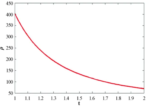
From Figure 1 one can easily see that energy density is decreasing with evolution of the universe. On differentiating Equation (21), we get

1 1

1 1 1

3

e Dt n e Dt n . n

mC

B C

t

α

ρ ₋ − _{ −} − _+ −

= − _ + _

Figure 1. This figureshows variation of energy density ρ with respect to

cosmic time t. Here we consider B = 1, C = 1, n = 1.5, m = 2 and α =1.

Now with the help of Equations (17)-(19) and (21), Equation (8) becomes

2 1

2 2

1

3 3 2

8π exp .

1 n n m mt G n t K

ρ+ Λ = − _− − _

−

  (23)

Which on differentiation yields

2 1

2 1 2

1

6 6 2

8π 8π exp ,

1

n

n n

m n m mt

G G

n

t K t

ρ+ ρ+ Λ =− ₊ + _− − _

−

 

 _  ₍₂₄₎

With the help of Equations (12), (14), (17)-(18) and (21), Equation (24) becomes

2 1

2 2 1

1

9 6 1 2

8π exp ,

1

n

n n n

m m mt mn

G

n

t t K t

η

ρ  − ₊ 

   

+ =  − − 

  _{ − }

      (25)

By use of Equations (15), (21) and (22) in Equation (25), we get

(

)

(

)

1 1 1

1 1

1 1

1 0 1

2 1

1

3

1 1 2

exp e e e ,

4π 1

n n n

r n

Dt Dt Dt

n n

m

mt mn

G C B C B C

n

K t t

α η α

− − − − − − + + − − − +    −   =   ₋ − − + + +            (26)

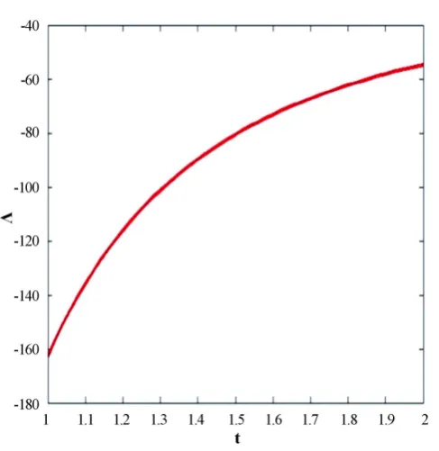
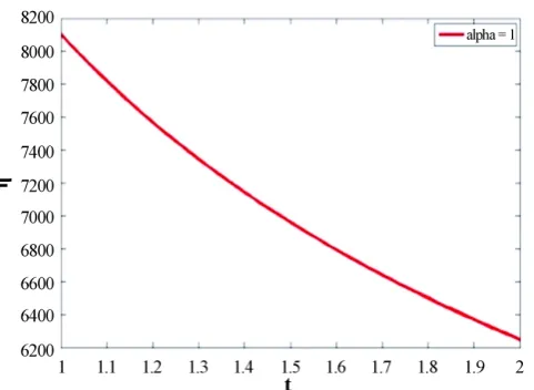
From Figure 2 it can be seen that G is increasing with evolution of the universe. Now using Equations (21) and (26) in Equation (23) gives

(

)

(

)

1 1 1

2 1 1

2 2 2 1

1 1 1 1 1 1 0

3 3 2 1 2

exp 2 exp

1 1

3

e n e n e n

n n

n n

r

Dt Dt Dt

n

m mt mt mn

n n

t K K t

m

C B C B C

t α η − − − − − + − − − + − − −   −  − 

Λ = − _{ }− _{  }− _

− _ − _         ⋅ − + + +      (27)

Figure 3 shows that cosmological constant is decreasing with the evolution of the universe.

On solving Equations (21) and (15) we can obtain the expression for bulk viscosity coefficient as

1 ₁

0 e .

n

r Dt

B C α

η η _{ −} − _{ +}

Figure 2. This figure shows variation of gravitational constant with respect to cosmic time t. Here we consider B = 1, C = 1, n = 1.5, m = 2, α =1, r =

1.5, a = 1 and η0=1.

Figure 3. This figure shows variation of cosmological constant with respect to cosmic time t. Here we consider B = 1, C = 1, n = 1.5, m = 2, α =1, r =

1.5, a = 1 and η₀=1.

Figure 4 shows that bulk viscosity coefficient is decreasing with evolution of the universe.

Thus the metric (1) reduces into the form

(

)

1

2 2 2 2 2 2 2 2 2

d d exp d e d e d .

1

n

k k

mt

s t K x y z

n

−

 

= − +  ₋  + +

  (29)

The deceleration parameter is given by

2

1 H

q

H

Figure 4. This figure shows variation of bulk viscosity coefficient with respect to cosmic time t. Here we consider B = 1, C = 1, n = 1.5, m = 2,

1

α = , r = 1.5 and η0=1.

1

1 n _n

q

mt−

= − + (30)

Expansion scalar, Shear coefficient, relative anisotropy for this model is given by

3 3

n

H m

H t

Θ =  = (31)

2

2 2 ₂

2 1 2 3

1 2 3

1

2 6

R

R R

R R R

σ = _ _ +_ _ +_ _ −Θ _{     } 

 



 

2 ₀

σ = (32) 2

Relative anisotropy σ 0

ρ

= = (33)

The critical energy density and the critical vacuum energy density are respectively given by

2

3 ,

8π 8π

c

H

G ν G

ρ = ρ = Λ

for the anisotropic Bianchi type V model can be expressed respectively as

(

)

(

)

1 1 1

2 2

1 1

1 1

1 0 1

2 1 1 3 , 3 1 2

2 exp e e e

1

n n n

n c

r n

Dt Dt Dt

n n

m t

m

mt mn

C B C B C

n

K t t

α α ρ η − − − − − − − + + − − − + =    −   − − + + +     ₋       _{ }  (34)

(

)

(

)

(

)

1 1 1

1 1

1 1

2 1 1 1

1 0

2 2 2 1

1 1 1 1 1 1 0 2 1 1 3

3 3 2 1 2

exp 2 exp e e e

1 1

3

1 2

2 exp e e e

1

n n n

n n

v

r

n n

Dt Dt Dt

n n n

n

Dt Dt

n n

m

m mt mt mn

C B C B C

n n

t K K t t

m

mt mn

C B C B C

n

K t t

α α ρ η η − − − − − − − − − − + − − − + − − + − − − + =     −  −  −  ₋ −   ₋ − − + + +             − ₋  _{− + + +}    ₋     

(

)

Mass density parameter and the density parameter of the vacuum are given by , M c c ν ρ ρ

ρ Λ ρ

Ω = Ω =

for the anisotropic Bianchi type V model can be expressed respectively as

(

)

(

)

1

1 1 1

1 ₁ 1 2 2 1 1 1 1 1 1 2 0 1 2

2 e exp

1

3

3 e e e

n

n n n

n

n Dt

n

M _r

Dt Dt Dt

n

mt mn

t B C

n

K t

m

m C B C B C

t

α

α η α

− − − − − + − + − + + − − −  −    ₊  _{  − }   _{ } − _{ } Ω =   − + + +       (36)

(

)

(

)

1 1 1

2 2 1 1

2 2 2 2 1

1 1 1 1 1 1 0

3 3 2 1 2

exp 2 exp

1 1

3

3

e n e n e n

n n n

n n

r

Dt Dt Dt

n

t m mt mt mn

n n

m t K K t

m

C B C B C

t α η − − − − − Λ + − − − + − − −  −   −  

Ω = _ −  ₋ −   ₋ − 

           _{ } ⋅ − + + +  _    _{ } (37)

The State finder parameters r R₃ RH

=  and 1

1 3 2 r s q − =  ₋      .

For this model

(

)

1 2 2 2

1 3

1 n_n n n _n

r

mt− m t −

+

= − + (38)

(

)

2 1

2 1 6

9 6

n n

n n t mn

s

m t mn

−

−

+ − =

− − (39)

3.2. Case II: Causal Cosmological Solution

In addition to physically plausible relations (15)-(17), in this case we assume

2

.

H β

Λ = (40) where H is Hubble parameter, given by

(

)

1 2 3

and .

R

H R R R R

R

=  = (41)

From Equation (17)-(19) and (41), the Hubble parameter is given by

n

m H

t

= (42)

Using equations (17)-(19), (40) and (42) in equation (8), we get

(

)

2 2

1

3 3 2

8π exp ,

1 n n m mt G n t K β

ρ= − − − ₋ − 

  (43) From Equations (21) and (43),

(

)

(

)

(

)

1 1 1

1 2 2 1 3 1 3 exp exp 8π n n n

G B C Dt D t

t K α β − − +  − −    = _ + − _{ } − _

  (44)

where 1

From Figure 5 one can easily see that gravitational constant is increasing with cosmic time. Substitute the values from Equations (17)-(19), (40) and (44) in Equation (5), we get

(

)

₍

₎

1 1

2 1 2

1

3 2 1 1

exp ,

8π

n

n n

m mn B

D t

G

t t K α

β

ρ −

+

 −  −

Π = − − ⋅ +

 

  (45)

By use of Equation (21), Equation (44) gives

(

)

( )

( )

(

)

1

1 1 1

2 1 1 exp exp n n U t B

B C Dt

U t

B C Dt

α α α − + − +  

Π = − _ + − _

 _{+ −} 

 

(46)

where

( ) (

)

(

)

2

1

1 2 1 2 1

1

3 2 1

exp n

n n

m mn

U t D t

t t K

β − +  −  = − −     ,

( ) (

)

₍

₎

2 2 2 1

1

3 3

exp n

n

U t D t

t K β − −   =_ − _  

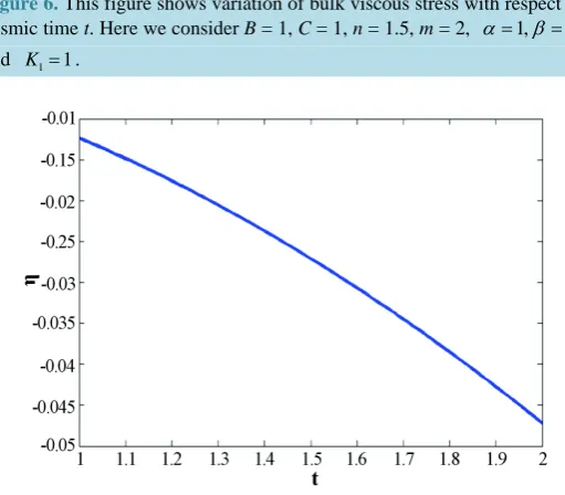
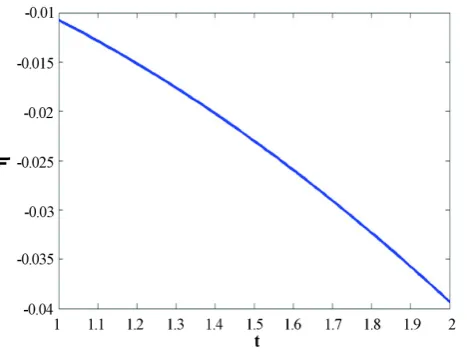
Figure 6 shows that bulk viscous stress is decreasing with the evolution of the universe.

3.2.1. Sub Cease (i): Evaluation of Bulk Viscosity in Truncated Causal Theory

Now we study variation of bulk viscosity coefficient η and relaxation time τ with respect to the cosmic time. It has already been mentioned that for truncated theory ε =0 and hence Equation (13) reduces to

3 H.

τ η

Π + Π = − (47) In order to have exact solution of the system of equations one more physically plausible relation is required. Thus, we consider the well known relation

. η τ

ρ

= (48)

Using Equations (17)-(19), (46) and (48) in Equation (47) one can obtain coefficient of bulk viscosity as

(

)

( )

( )

(

)

( )

( )

( ) ( )

_{( )}

( )

( )

(

)

(

)

(

)

(

)

1 1 1 1

1 2

1

1 1 2 1 1 1

2

2 ₂ 2

2 1 1 exp exp 3 exp exp 3 3 exp exp n n n n n n n n n

B B C Dt U t U t B C Dt

U t U t U t U t mC

Dt B C Dt

U t _{U t} U t t

BCm m

Dt B C Dt

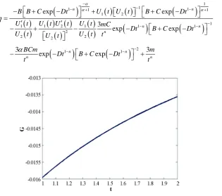
t t α α α η α − − − + − + − − − − − −     − _ + − _ + _ _{ } + − _ = ′ ′   − + − − _ + − _       − − _ + − _ + (49)

Figure 5. This figure shows variation of gravitational constant with respect to

Figure 6. This figure shows variation of bulk viscous stress with respect to cosmic time t. Here we consider B = 1, C = 1, n = 1.5, m = 2, α=1,β=1, and K₁=1.

Figure 7. This figure shows variation of bulk viscosity coefficient with respect

to cosmic time t. Here we consider B = 1, C = 1, n = 1.5, m = 2, α =1.

From Figure 7 one can see that bulk viscosity coefficient is decreasing with time.

3.2.2. Sub Caese (ii). Evaluation of Bulk Viscosity in Full Causal Theory

It has already been mentioned that for full causal theory ε =1 and hence Equation (13) reduces to

3 3 .

2

T

H H

T

τ τ η

τ η

τ η

 

Π

Π + Π = − − _ − − − _

 

  

 ₍₅₀₎

On the basis of Gibb’s inerrability condition, Maartens [40] has suggested the equation of state for tempera-ture as

d exp p ,

T

p ρ

∝

+

∫

( 1) 1

0 1 .

T T B

α α α ρ− + +

 

= _ − _ (52)

Figure 8 shows that temperature is decreasing with evolution of the universe.

using Equations (21), (42), (48) and (52) in Equation (50) one can obtain

1 2 1 2

2 2

, 2

n n

m m m m T

T

t t

η _η η ρ

ρ ρ ρ

 

+ Π +

Π + Π = − − _ − − _

 

  

which on simplification yields the expression for bulk viscosity as

(

)

( )

( )

(

)

(

)

(

)

( )

( )

(

)

(

)

(

)

(

)

(

)

1 1

1 1 1 1

1 2

1 1

1 1

2

exp exp

3 1 exp

3 1 3

exp exp

n n

n

n n n n n

B B C Dt U t U t B C Dt

mC Dt

U t m

m B

U t

t _{B C Dt} t _{t B C Dt}

α

α α

η

α α

ρ

−

−

− + − +

−

− −

   

− _ + − _ + _ _{ } + − _ =

   _{+ + −} 

Π    

+ + − +

 _{+ −}   _{+ −} 

   

 (53)

where

( )

( )

( ) ( )

_{( )}

( )

( )

(

)

(

)

(

)

(

)

1

1 1 2 1 1 1

2

2 ₂ 2

2

1 1

3

exp exp

3

exp exp

n n

n

n n

n

U t U t U t U t mC

Dt B C Dt

U t _{U t} U t t

BCm

Dt B C Dt

t ρ

α

−

− −

−

− −

′ ′

Π _{ }

= − + − − _ + − _

   

 

− − _ + − _



Figure 9 shows that bulk viscosity coefficient decreasing with evolution of universe.

4. Conclusion

In this paper, we have studied bulk viscous Bianchi type V space-time geometry with generalized Chaplygin gas and varying gravitational and cosmological constants. We have obtained a new set of exact solutions of

Einstein’s equations by considering 1 2

1 2

n

R R m

R =R =t

 

. For n > 1, the deceleration parameter q < 0 for

(

)

t> n m − _.

When n→1 considering present day limit for deceleration parameter 0.17 0.13

0.53

q= − +₋ [40] suggests

1.56≤m≤2.94. It is observed that in case I energy density, bulk viscosity and cosmological constant decrease where as gravitational constant G(t) is increasing with time. In case II, bulk viscosity η, bulk viscous stress Π and temperature T decrease with evolution of the universe which agrees with cosmic observations. In order to

Figure 8. This figure shows variation of temparature with respect to

Figure 9. This figure shows variation of bulk viscosity coefficient with respect to cosmic time t. Here we consider B = 1, C = 1, n = 1.5, m = 2,

1

α = .

have clear idea of variation in behavior of cosmological parameters, relevant graphs have been plotted; all graphs are in fair agreement with cosmological observations.

References

[1] Misner, C.W. (1968) The Isotropy of the Universe. Astrophysical Journal, 151, 431-457. http://dx.doi.org/10.1086/149448

[2] Farnsworth, D.L.(1967)Some New General Relativistic Dust Metrics Possessing Isometries. Journal of Mathematical Physics, 8, 2315. http://dx.doi.org/10.1063/1.1705157

[3] Collins, C.B. (1974) Tilting at Cosmological Singularities. Communications in Mathematical Physics, 39, 131-151. http://dx.doi.org/10.1007/BF01608392

[4] Maartens, R. and Nel, S.D. (1978) Decomposable Differential Operators in a Cosmological Context. Communications in Mathematical Physics, 59, 273-283.

http://dx.doi.org/10.1007/BF01611507

[5] Wainwright, J., Ince, W.C. and Marshman, W. (1979) Spetially Himigeneous and Inhomogeneous Cosmologies with Equation of State p = μ. General Relativity and Gravitation, 10, 259-271.

http://dx.doi.org/10.1007/BF00759860

[6] Roy, S.R. and Singh, J.P. (1983) LRS Bianchi Type-V Universes Filled with Matter and Radiation. Astrophysics and Space Science, 96, 303-312. http://dx.doi.org/10.1007/BF00651674

[7] Banerjee, A. and Sanyal, A.K. (1988) Irrotational Bianchi Type V Viscous Fluid Cosmology with Heat Flux. General Relativity and Gravitation, 20, 103-113. http://dx.doi.org/10.1007/BF00759320

[8] Coley, A.A. (1990) Conformal Killing Vectors and FRW Spacetimes. General Relativity and Gravitation, 22, 241-251. http://dx.doi.org/10.1007/BF00756274

[9] Roy, S.R. and Prasad, A. (1994) Some L.R.S. Bianchi Type V Cosmological Models of Local Embedding Class One.

General Relativity and Gravitation, 19, 939-950. http://dx.doi.org/10.1007/BF02106663

[10] Nayak, B.K. and Sahoo, B.K. (1989) Bianchi Type V Model with the Matter Distribution Admitting Anisotropic Pres-sure and Heat Flow. General Relativity and Gravitation, 21, 211-225. http://dx.doi.org/10.1007/bf00764095

[11] Bali, R. and Meena, B.L. (2004) Conformally Flat Tilted Bianchi Type-V Cosmological Models in General Relativity.

Pramana: Journal of Physics, 62, 1007-1014.

[12] Bali, R. and Yadav, M.K. (2005) Bianchi Type-IX Viscous Fluid Cosmological Model in General Relativity. Pramana:

Journal of Physics, 64, 187-196.

[13] Bali, R. and Singh, D.K. (2005) Bianchi Type V Bulk Viscous Fluid String Dust Cosmological Model in General Rela-tivity. Astrophysics and Space Science, 300, 387-394.

[15] Rajbali, S.T. (2008) Bianchi Type V Bulk Viscous Barotropic Fluid Cosmological Models with Variable G and Lamb-da. Chinese Physics Letters, 25, 3090-3093. http://dx.doi.org/10.1088/0256-307X/25/8/095

[16] Yadav, A.K. (2013) Anisotropic Massive Strings in the Scalar Tensor Theory of Gravitation. Research in Astronomy and Astrophysics, 13, 772-782. http://dx.doi.org/10.1088/1674-4527/13/7/002

[17] Yadav, A.K., Pradhan, A. and Singh, A.K. (2012) Bulk Viscous LRS Bianchi Type I Universe with Variable G and Lambda. Astrophysics and Space Science, 337, 379-385. http://dx.doi.org/10.1007/s10509-011-0814-7

[18] Ellis, G.F.R. (1979) In: Schas, R., Ed., General Relativity and Cosmology, Enrico Fermi Course, Academic Press, New York, 47. Misner, C.W. (1968) The Isotropy of the Universe. Astrophysical Journal, 151, 431.

[19] Fabris, J.C., Concalves, S.V.B. and de Sa’Ribeiro, R. (2006) Bulk Viscosity Driving the Acceleration of the Universe.

General Relativity and Gravitation, 38, 495-506. http://dx.doi.org/10.1007/s10714-006-0236-y

[20] Kotambkar, S., Singh, G.P. and Kelkar, R.K. (2014) Anisotropic Cosmological Models with Quintessence. Interna-tional Journal of Theoretical Physics, 53, 449-460. http://dx.doi.org/10.1007/s10773-013-1829-3

[21] Krauss, L.M. and Turner, M.S. (1995) The Cosmological Constant Is Back. General Relativity and Gravitation, 27, 1137-1144. http://dx.doi.org/10.1007/bf02108229

[22] Riess, A.G., Filippenko, A.V., Challis, P., Clocchiatti, A., Diercks, A., Garnavich, P.M., et al. (1998) Observational Evidence from Supernovae for an Accelerating Universe and a Cosmological Constant. The Astronomical Journal, 116, 1009-1038. http://dx.doi.org/10.1086/300499

[23] Perlmutter, S., Aldering, G., Goldhaber, G., Knop, R.A., Nugent, P., Castro, P.G., et al. (1999) Measurements of Omega and Lambda from 42 High Redshift Supernovae. The Astronomical Journal, 517, 565-586.

http://dx.doi.org/10.1086/307221

[24] Lima, J.A.S. and Trodden, M. (1996) Decaying Vacuum Energy and Deflationary Cosmology in Open and Closed Universe. Physical Review D, 53, 4280-4286. http://dx.doi.org/10.1103/physrevd.53.4280

[25] Bennett, C.L., Halpern, M., Hinshaw, G., Jarosik, N., Kogut, A., Limon, M., et al. (2003) First Year Wilkinson Mi-crowave Anisotropy Prob (WMAP) Observations—Preliminary Maps and Basic Results. Astrophysical Journal Sup-plement, 148, 1-27.

[26] Sahni, V. and Starobinski, A. (2000) The Case for a Positive Cosmological Lambda Term. International Journal of Modern Physics D, 9, 373-444.

[27] Canuto, V.M. and Narlikar, J.V. (1980) Cosmological Tests of the Hoyle-Narlikar Conformal Gravity. The Astrophys-ical Journal, 236, 6-23. http://dx.doi.org/10.1086/157714

[28] Singh, G.P. and Kotambkar, S. (2001) Higher Dimensional Cosmological Model with Gravitational and Cosmological “Constants”. General Relativity and Gravitation, 33, 621-630. http://dx.doi.org/10.1023/A:1010278213135

[29] Singh, G.P. and Kotambkar, S. (2003) Higher Dimensional Dissipative Cosmology with Varying G and Lambda. Gra-vitation and Cosmology, 9, 206-210.

[30] Singh, G.P., Kotambkar, S. and Pradhan, A. (2008) A New Class of Higher Dimensional Cosmological Models of Un-iverse with Variable G and Lambda Term. Romanian Journal of Physics, 53, 607-618.

[31] Pradhan, A. and Pandey, P. (2006) Some Bianchi Type I Viscous Fluid Cosmological Models with a Variable Cosmo-logical Constant. Astrophysics and Space Science, 301, 127-134.

Pradhan, A., Singh, A.K. and Otarod, S. (2007) FRW Universe with Variable G and Lambda Term. Romanian Journal of Physics, 52, 445-458.

[32] Singh, C.P. and Kumar, S. (2006) Bianchi Type II Cosmological Models with Constant Deceleration Parameter. Inter-national Journal of Modern Physics D, 15, 419-438. http://dx.doi.org/10.1142/s0218271806007754

[33] Singh, C.P., Kumar, S. and Pradhan, A. (2007) Early Viscous Universe with Variable Gravitational and Cosmological Constant. Classical and Quantum Gravity, 24, 455-474. http://dx.doi.org/10.1088/0264-9381/24/2/011

[34] Singh, J.P. and Tiwari, S.K. (2008) Perfect Fluid Bianchi Type I Cosmological Constant Models with Time Varying G and Lambda. Pramana, 70, 565-574.

[35] Singh, G.P. and Kale, A.Y. (2009) Anisotropic Bulk Viscous Cosmological Models with Variable G and Lambda. In-ternational Journal of Theoretical Physics, 48, 1177-1185. http://dx.doi.org/10.1007/s10773-008-9891-y

[36] Bali, R. and Tinkar, S. (2009) Bianchi Type III Bulk Viscous Barotropic Fluid Cosmological Models with Variable G and Lambda. Chinese Physics Letters, 26, Article ID: 029802. http://dx.doi.org/10.1088/0256-307X/26/2/029802 [37] Verma, M.K. and Ram, S. (2011) Spatially Homogeneous Bulk Viscous Fluid Models with Time-Dependent

Gravita-tional Constant and Cosmological Term. Advanced Studies in Theoretical Physics, 5, 387-398.

[39] Bento, M.C., Bertolami, O. and Sen, A.A. (2003) WMAP Constraints on the Generalized Chaplygin Gas Model. Phys-ics Letters B, 575, 172-180. http://dx.doi.org/10.1016/j.physletb.2003.08.017