Periodically Disturbed Oscillators

(1)

Thesis by

Brian Daffern Hong

In Partial Fulfillment of the Requirements for the Degree of

Doctor of Philosophy

CALIFORNIA INSTITUTE OF TECHNOLOGY Pasadena, California

2019

(2)

Brian Daffern Hong ORCID: 0000-0001-8099-0312

(3)

(4)

ACKNOWLEDGEMENTS

Without a doubt, attending graduate school has been the most tumultuous time of

my life thus far. As a younger student, it has also served as a period of tremendous

personal and academic growth. As I write this, I am still amazed by the factors and

decisions that led me to where I am today, and it still feels surreal looking back on many of the events that have occurred in the past couple years.

I owe an immeasurable amount of gratitude to my advisor, Professor Ali Hajimiri.

He is, of course, academically brilliant, but what sets him apart is how deeply he

cares for his students on a personal level. With us, he wears many hats. As a

stern academic advisor, he nurtures and motivates our intellectual growth. As a life

mentor, he imparts wisdom into the non-academic aspects of our existence. As a

father figure, he comforts us through the many ups and downs of our lives. As a friend, he takes us on group outings and chats with us about the myriad of topics for

which he is eminently knowledgeable—from food and cinema to sports and history.

More personally, I know that I was not by any means an easy student to advise. Yet,

not only did Ali serve as a consistent pillar of emotional support, he also looked past

my immaturity, gave me many more chances than I deserved, patiently provided me

with space and time for me to work through my personal struggles, and continued

to believe in me even when I had given up on myself. There are few people in the

world like Ali, and working with him has been a once-in-a-lifetime opportunity.

Next, I would like to express my appreciation to Professors Azita Emami, P. P.

Vaidyanathan, and Changhuei Yang for serving on my thesis committee, and also

to Professor Babak Hassibi who could not make it to my defense but served on my

candidacy committee. In the short amount of time they had to evaluate my work,

they intently provided me with valuable feedback on how best to improve it.

It goes without saying that this work could not have been completed without the

constant support from my colleagues. Aroutin Khachaturian, who has been my

labmate the longest, emanates a kindness that knows no bounds and a generosity matched only by his awe-inspiring work ethic. I have treasured every single one

of our many late-night journeys in search of boba and random food to snack on.

Dr. Alex Pai, my “brother from another mother” and “partner in crime,” has been

there for me countless times. He helped me pick myself up in the face of seeming

(5)

It is not an understatement to say that I have learned much about life in general from

him. Abhinav Agarwal is my “brother from another circuits lab.” Our many dinners sampling the best Indian food LA has to offer and bonding over the difficulties of

research always left me reinvigorated. My good friend Parham ‘Parjom’ Porsandeh

Khial is driven by a fierce idealism and ambition which has never ceased to inspire

me. I will miss our stress-relieving trips to Mammoth, Big Bear, and Las Vegas.

Dr. Constantine ‘Costis’ Sideris is a caring, thoughtful, and intelligent individual.

Oftentimes, a short conversation with him would enable me to make significant

progress in whatever issue I was struggling with, academic or otherwise. Reza

Fatemi has a rare gift: a sharp analytical mind combined with a uniquely profound

insight into human behavior. His gentle encouragement and shrewd advice pulled me out of several ruts, both within and outside of research. Matan Gal-Katziri’s

seasoned outlook on life intermittently provided me with indispensable doses of

maturity. Additionally, I am deeply grateful to him for his invaluable assistance

with several critical parts of my measurement setup. Alexander ‘Alex’ White’s

fearless enthusiasm and hands-on mindset often aided my research in unexpected

ways. Austin Fikes’ sardonic wit, comedic comments about politics, and ability

to find free food on campus served as refreshing injections into the day-to-day

frustrations of grad school. The deeply compassionate David ‘Elliott’ Williams

sympathizes with people of all plights; he connected with me during some of my darkest times. He also handled the unenviable task of coordinating with MOSIS for

the fabrication and delivery of my chips. Craig Ives has been my work buddy during

the numerous all-nighters I pulled in the past year, occasionally providing me with

respite through impromptu conversations about philosophy and psychology. Dr.

Kaushik Dasgupta’s technical acumen and lightheartedness made me realize that

things are not always as hard as they initially seemed. Stefan Turkowski’s love of

live music and ability to cook awesome food gave me a way to unwind outside of

the lab. I will also never forget our transformative experience backpacking through

Southeast Asia. Finally, I would like to thank Dr. Behrooz Abiri, Dr. Florian Bohn, Prof. Steve Bowers, Dr. Amirreza ‘Amir’ Safaripour, Dr. M. Reza Hashemi,

Kuan-Chang ‘Xavier’ Chen, Milad Taghavi, and Aryan Hashemi for their friendship and

support.

Outside of the 3rd floor of Moore, several close confidantes have kept me sane and

grounded throughout my time at Caltech. My dear friends Corina Bianca Panda,

Surabhi Sachdev, and Dr. Ramya Korlakai Vinayak helped me see the light when

(6)

understanding my feelings in a way that no one else could. The sea of empathy

that swells within Surabhi’s heart always drowned out my feelings of emptiness and loneliness. From Ramya, I have learned not to lose hope in spite of life’s

unpredictability and complexity. Utkan Onur Candoˇgan’s wry humor juxtaposed

against his practical sensibilities helped me recognize when I was taking things

too seriously. Katherine Rinaldi and Annalise ‘Anna’ Sundberg showed me the

importance of maintaining balance in the midst of overwhelming stress. Lastly,

I would like to mention my other friends at Caltech who have helped to relieve

the burden of graduate school: Dr. Betty Ko Wong, Tahmineh ‘Tami’ Khazaei,

Aubrey Shapero, Dr. Maria Sakovsky, Fariborz Salehi, Maxim ‘Max’ Budninskiy,

and Armeen Taeb.

Beyond Caltech, a few lifelong confidantes deserve recognition as well. My chance

encounter with Joy Dou at the Buddhist temple we go to blossomed into a

friend-ship filled with adventures—from the turquoise waters of the Havasupai Indian

Reservation to the red canyons of Zion National Park and the summit of Mount

Whitney—which always rejuvenated me with happiness. Anthony Chan’s humility,

kindness, and humor reminded me to appreciate the small things in life. Dr. Angie

Wang brightened my holidays by accompanying me to Disneyland and inviting me

to her house for Christmas. I am thankful to Pak-Ling ‘Leo’ Szeto for providing me with a second family (IEEE) during my time as an undergraduate at UCLA and

serving as a source of emotional stability throughout my graduate studies at Caltech.

The many dinners I enjoyed, movies I watched, and (ironically) clinical discussions

about depression I had with Michael Sechooler always left me feeling less weighed

down by the world. Kamal Kajouke provided me with a shoulder to cry on whenever

things were not going as expected. Finally, I am grateful to my other friends from

undergrad, Calvin Cam, Justin Young, Shubham Gandhi, and Minh-Trang ‘Teresa’

Ha, for staying in touch and keeping it real as I slaved away in the ivory tower.

Next, I want to acknowledge the MICS lab for lending me equipment for my

experi-ments, as well as David Hodge, Michelle Chen, Tanya Owen, Carol Sosnowski, and

Christine Garske, for doing much of the work behind the scenes to ensure the smooth

operation of our lab and our department. I would also like to convey my utmost

appreciation to the Dean of Graduate Studies at Caltech, Professor Douglas Rees,

and Assistant Dean Natalie Gilmore for their continued support in my endeavor to

complete my PhD. Last but not least, I am grateful to the Admissions Office at Yale

(7)

In closing, I am indebted to my parents for raising me and for being an infinite

source of guidance and love throughout my life. I owe them mine many times over.

This work was partially supported by the Air Force Office of Scientific Research

(AFOSR), under Multidisciplinary Research Program of the University Research

(8)

ABSTRACT

By controlling the timing of events and enabling the transmission of data over

long distances, oscillators can be considered to generate the “heartbeat” of modern

electronic systems. Their utility, however, is boosted significantly by their peculiar

tendency to synchronize to external signals that are themselves periodic in time. Although this fascinating phenomenon has been studied by scientists since the

1600s, models for describing this behavior have seen a disconnect between the

rigorous, methodical approaches taken by mathematicians and the design-oriented,

physically-based analyses carried out by engineers. While the analytical power of

the former is often concealed by an inundation of abstract mathematical machinery,

the accuracy and generality of the latter are constrained by the empirical nature of

the ensuing derivations. We hope to bridge that gap here.

In this thesis, a general theory of electrical oscillators under the influence of a

periodic injection is developed from first principles. Our approach leads to a

fun-damental yet intuitive understanding of the process by which oscillators lock to

a periodic injection, as well as what happens when synchronization fails and the

oscillator is instead injection pulled. By considering the autonomous and

periodi-cally time-varying nature that underlies all oscillators, we build a time-synchronous

model that is valid for oscillators of any topology and periodic disturbances of any

shape. A single first-order differential equation is shown to be capable of making

accurate, quantitative predictions about a wide array of properties of periodically

disturbed oscillators: the range of injection frequencies for which synchronization occurs, the phase difference between the injection and the oscillator under lock,

stable vs. unstable modes of locking, the pull-in process toward lock, the dynamics

of injection pulling, as well as phase noise in both free-running and injection-locked

oscillators. The framework also naturally accommodates superharmonic

injection-locked frequency division, subharmonic injection-injection-locked frequency multiplication,

and the general case of an arbitrary rational relationship between the injection and

oscillation frequencies. A number of novel insights for improving the performance

of systems that utilize injection locking are also elucidated. In particular, we

ex-plore how both the injection waveform and the oscillator’s design can be modified to optimize the lock range. The resultant design techniques are employed in the

im-plementation of a dual-moduli prescaler for frequency synthesis applications which

(9)

For the commonly used inductor-capacitor (LC) oscillator, we make a simple

mod-ification to our framework that takes the oscillation amplitude into account, greatly enhancing the model’s accuracy for large injections. The augmented theory uniquely

captures the asymmetry of the lock range as well as the distinct characteristics

ex-hibited by different types of LC oscillators. Existing injection locking and pulling

theories in the available literature are subsumed as special cases of our model. It

is important to note that even though the veracity of our theoretical predictions

degrades as the size of the injection grows due to our framework’s linearization with

respect to the disturbance, our model’s validity across a broad range of practical

injection strengths are borne out by simulations and measurements on a diverse

collection of integrated LC, ring, and relaxation oscillators. Lastly, we also present a phasor-based analysis of LC and ring oscillators which yields a novel perspective

into how the injection current interacts with the oscillator’s core nonlinearity to

(10)

PUBLISHED CONTENT AND CONTRIBUTIONS

[1] B. Hong and A. Hajimiri, “A general theory of injection locking and pulling in electrical oscillators—Part I: Time-synchronous modeling and injection waveform design,” IEEE Journal of Solid-State Circuits, vol. 54, no. 8, pp. 2109–2121, Aug. 2019. doi:10.1109/JSSC.2019.2908753,

B. Hong conceived of the project, conducted all of the research, and authored the manuscript.

[2] ——, “A general theory of injection locking and pulling in electrical oscillators—Part II: Amplitude modulation in LC oscillators, transient be-havior, and frequency division,”IEEE Journal of Solid-State Circuits, vol. 54, no. 8, pp. 2122–2139, Aug. 2019. doi:10.1109/JSSC.2019.2908763, B. Hong conceived of the project, conducted all of the research, and authored the manuscript.

[3] ——, “A phasor-based analysis of sinusoidal injection locking in LC and ring oscillators,”IEEE Transactions on Circuits and Systems I: Regular Papers, vol. 66, no. 1, pp. 355–368, Jan. 2019. doi:10.1109/TCSI.2018.2860045, B. Hong conceived of the project, conducted all of the research, and authored the manuscript.

[4] ——, “Upper and lower bounds on a system’s bandwidth based on its zero-value time constants,” Electronics Letters, vol. 52, no. 16, pp. 1383–1385, Aug. 2016. doi:10.1049/el.2016.1724,

[5] ——, “Analysis of a balanced analog multiplier for an arbitrary number of signed inputs,” International Journal of Circuit Theory and Applications, vol. 45, no. 4, pp. 483–501, Apr. 2017. doi:10.1002/cta.2243,

[6] A. Pai, P. Cao, E. E. White, B. Hong, M. Wang, B. Badie, A. Hajimiri, and J. M. Berlin, “Dynamically programmable magnetic fields for controlled movement of cells loaded with iron oxide nanoparticles,” submitted to Bio-conjugate Chemistry,

(11)

12.2 Holistic Design of Multi-Phase Switched-Capacitor DC-DC Con-verters with a Large Number of Conversion Ratios . . . 243 Bibliography . . . 250 Appendix A: Measurement Setup . . . 264 Appendix B: The Problem with the Single-Period Injection Response (SPIR) . 268 Appendix C: Miscellaneous Mathematical Facts . . . 278 C.1 Some Standard Integrals . . . 278 C.2 Proof of Claim 8.4.1 . . . 278 Appendix D: Correction to “A Study of Injection Locking and Pulling in

(14)

LIST OF ILLUSTRATIONS

Number Page

1.1 Arbitrary electromagnetic surface featuring multiple voltage-controlled

oscillators (VCOs) that drive the radiating elements. . . 2

1.2 Mathematical description of an oscillator as traversing a stable limit

cycle inndimensions. Points in the state space not on the orbit will

eventually converge to the limit cycle. . . 3

1.3 A basic cartoon of the setup and notation underlying the analysis. In

the free-running case (i.e.,iinj = 0), ξ(t)= 0 andϕ(t)= ω0t. Under

injection, the phase becomes ϕ(t) ≡ω0t+φ(t) ≡ωinjt+θ(t). . . 4 1.4 An example of injection locking. Note that the oscillation voltage is

observed at the node being injected into. . . 6

1.5 An example of injection pulling where f0=1 GHz and finj =0.8 GHz. 7

1.6 Zooming into a single “beat” for the injection-pulled oscillator of

Figure 1.5. . . 8

2.1 Schematic of the basic LC oscillator under injection used in the

derivation of Adler’s equation. . . 12

2.2 A nonlinear model of the ring oscillator often used for injection locking and pulling applications. . . 15

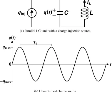
3.1 Idealized conceptual setup for our thought experiment. . . 19

3.2 Synchronizing an LC tank to an impulse train of current injections

which leave the amount of energy in the tank unchanged. . . 21

3.3 Applying an impulse train current injection to an LC oscillator. We

are interested in the steady-state behavior of this circuit. . . 22

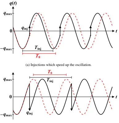
3.4 Varying the time at which the injections are applied. . . 23

3.5 Defining the phaseθusing the fundamental components of the wave-forms from Figure 3.4. . . 24 3.6 Depiction of how the oscillation amplitudeqmax(t)evolves with time

in steady-state when the injections change the amount of energy stored

in the tank. . . 26

4.1 Relating the time-varying impulse response for the oscillator’s excess

(15)

4.2 The impulse sensitivity function (ISF) captures the dependence of

the incurred phase shift on the time of injection. . . 31 4.3 Block diagram depicting what happens to the phase of a periodically

disturbed oscillator. . . 37

4.4 Decomposing the ISF into its spectral components, emphasizing how

the injection waveform is filtered in the formation of the lock

charac-teristic. . . 38

4.5 Schematic of the comparator-based relaxation oscillator. . . 40

4.6 Time shift ∆TD induced by an injection into a Bose oscillator while

it is discharging. . . 41

4.7 One period of the free-running oscillation voltage of an ideal, sym-metric 1 GHz Bose oscillator withVDD =VSS= 1 V. . . 43

4.8 The impulse sensitivity function of the ideal Bose oscillator (whose

oscillation voltage is shown in Figure 4.7) obtained several different

ways. . . 44

4.9 Exploring the effect of injecting a DC current into one of the stages

of a 1 GHz 17-stage ring oscillator. . . 46

4.10 3-stage single-ended inverter-chain ring oscillator. . . 48

4.11 Lock characteristic of the 3-stage ring oscillator for sinusoidal

injec-tions of varying amplitudeIinj. . . 49

4.12 17-stage single-ended inverter-chain ring oscillator. . . 50

in-jections of varying amplitudeIinj. . . 51

4.14 6-stage differential ring oscillator. . . 52

4.16 Lock characteristic of the ideal Bose oscillator for sinusoidal

4.17 NMOS differential astable multivibrator. . . 56 4.18 Lock characteristic of the astable multivibrator oscillator for

sinu-soidal injections of varying amplitude Iinj. . . 57

4.19 Die photo of the measured oscillators. Pads for the supply (‘VDD’) of

each oscillator, ground (‘GND’), and the injections (‘INJP’,‘INJN’)

are labeled. . . 59

4.20 Measurement results for the 3-stage single-ended ring oscillator. . . . 60

(16)

4.22 Measurement results for the 6-stage differential ring oscillator. . . 62

4.23 Measurement results for the Bose oscillator. . . 64 4.24 Measurement results for the differential astable multivibrator. . . 65

5.1 An example of how the injection could alter the oscillation amplitude. 67

5.2 The phase shift ∆ϕ induced by the injection of charge qinj depends inversely on the maximum charge swingqmaxacross the capacitor. . . 69

5.3 The dynamic by which the oscillator dissipates excess energy is

cap-tured by the decay function D(·,·). . . 70 5.4 Relating the time-varying impulse response for orbital deviations to

the amplitude ISF and the APF. . . 73

5.5 The APF captures the perturbation in the oscillation amplitude caused by the injection—for which the ISF of an LC oscillator has an inverse

dependence. . . 74

5.6 Cross-coupled CMOS differential LC oscillator. . . 77

5.7 Other properties of the cross-coupled CMOS differential LC oscillator. 78

5.8 Predicted and simulated behavior of a sinusoidally injection-locked

CMOS differential LC oscillator with an injection amplitude ofIinj =

0.5 mA. . . 79 5.9 Predicted and simulated behavior of a sinusoidally injection-locked

0.75 mA. . . 80 5.10 Predicted and simulated behavior of a sinusoidally injection-locked

1 mA. . . 81

2 mA. . . 82

5.12 Cross-coupled NMOS-only differential LC oscillator. . . 83

5.13 Other properties of the NMOS-only differential LC oscillator. . . 84 5.14 Predicted and simulated behavior of a sinusoidally injection-locked

NMOS-only differential LC oscillator with an injection amplitude of

Iinj =0.5 mA. . . 85 5.15 Predicted and simulated behavior of a sinusoidally injection-locked

(17)

Iinj =1 mA. . . 87 5.17 Predicted and simulated behavior of a sinusoidally injection-locked

Iinj =2 mA. . . 88

5.18 Common-base bipolar Colpitts oscillator. . . 89

5.19 Other properties of the common-base bipolar Colpitts oscillator. . . . 90

Colpitts oscillator with an injection amplitude ofIinj =2.5 mA. . . . 91

5.21 Predicted and simulated behavior of a sinusoidally injection-locked Colpitts oscillator with an injection amplitude ofIinj =5 mA. . . 92

Colpitts oscillator with an injection amplitude ofIinj =10 mA. . . 93

5.23 Die photo of the measured oscillators. The supply (‘VDD’) pads

for each oscillator as well as the ground (‘GND’) and injection

(‘INJP’,‘INJN’) pads are labeled. . . 94

5.24 Lumped-element model for an on-chip symmetric spiral inductor

[97]–[99]. Cs andrsare the series capacitance and resistance,Coxis

the capacitance across the oxide, andCSi, andRSiare the capacitance

and resistance of the silicon substrate. . . 95

5.25 Schematic of the common-gate MOS Colpitts oscillator. A resistively

biased current mirror and a resistive divider generate Ibias and Vb,

respectively. . . 96

5.26 Measurement results for the CMOS differential LC oscillator. . . 99

5.27 Measurement results for the NMOS-only differential LC oscillator. . 100

5.28 Measurement results for the MOS Colpitts oscillator. . . 101

5.29 Behavioral model of an ideal, current-biased LC oscillator with a

sinusoidal injection. . . 102 5.30 Equivalence between the thought experiment of Chapter 3 and the

time-synchronous model of Chapters 4 and 5. . . 109

6.1 Injection into the tail node of a CMOS differential LC oscillator. . . . 112

6.2 Lock characteristic of the differential LC oscillator for a sinusoidal

injection at the 2nd harmonic into the tail node. . . 113

6.3 Lock characteristic of the 17-stage single-ended ring oscillator for a

(18)

6.4 7-stage asymmetric ring oscillator withWN/WP =3. . . 115 6.5 Lock characteristic of the 7-stage single-ended asymmetric ring

os-cillator for aIinj =0.25 mA sinusoidal injection at the first 5 harmonics.117 6.6 Lock characteristic of the ideal Bose oscillator for a 5 mA sinusoidal

injection at the 3rd harmonic. . . 118

6.7 Die photo of the measured oscillators. The supply (‘VDD’) pads

for each oscillator, the ground (‘GND’) pad, the differential injection

(‘INJP’,‘INJN’) pads, and the tail injection (‘INJT’) pad are labeled. . 119

6.8 Superharmonic lock range measurement results for two different ring

oscillators. . . 122

6.9 Superharmonic lock range measurement results for the 10 MHz Bose relaxation oscillator. . . 124

6.10 Superharmonic lock range measurement results for the NMOS

dif-ferential astable multivibrator. . . 125

6.11 Schematic of the NMOS-only differential LC oscillator with a tail

injection. Itailis implemented with a resistively biased current mirror. 126

6.12 Measurement results for injecting into the tail of the CMOS

differen-tial LC oscillator. . . 127

6.13 Measurement results for injecting into the tail of the NMOS-only

differential LC oscillator. . . 128 6.14 Generalization of Figures 4.3 and 4.4 to allow for M:N

sub-/super-harmonic injection locking and pulling. . . 132

6.15 A ring oscillator with an injection applied to every stage.

Differen-tial ring oscillators consisting of an even number of stages have an

additional inversion in the feedback path. . . 133

6.16 Multi-phase injection lock characteristic of the 7-stage single-ended

asymmetric ring oscillator for a sinusoidal injection at the first 5

harmonics. . . 137

6.17 Example calculations of θ for a 2nd harmonic sinusoidal injection into the tail of a differential LC oscillator. The phases φinjand φosc are computed assuming the time reference t0 starts at the beginning of the depicted window. . . 141

6.18 A plot of the example oscillation voltage from Eq. (6.34) and injection

(19)

7.1 A feedback block diagram representation of fundamental pulling

equation. The ISF and the injection waveform govern the behav-ior of the lock characteristicΩ(θ). . . 146 7.2 A graphical viewpoint of the lock characteristic which shows the lock

range and stable vs. unstable regions. Note that the lock characteristic

is periodic with a period of 2π/N. . . 147 7.3 A block diagram showing how the injection waveform and the ISF

interact to form the pull-in frequency. . . 149

7.4 Simulated pull-in process of a sinusoidally injection-locked 17-stage

ring oscillator for two different injection amplitudes. . . 150

7.5 Simulated pull-in process of a sinusoidally injection-locked CMOS differential LC oscillator. . . 152

7.6 Two examples of the magnitude spectrum of an injection-pulled

17-stage ring oscillator. The free-running frequency is f0 =1.0013 GHz and the injection is sinusoidal with an amplitude ofIinj =1.5 mA. . . 156

7.7 Magnitude spectrum of a 1.0013 GHz 17-stage ring oscillator pulled by a 1.5 mA sinusoidal injection at 0.97 GHz. . . 157 7.8 Magnitude spectrum of a 1GHz Colpitts oscillator pulled by a 7.5mA

sinusoidal injection at 0.7 GHz. . . 158 7.9 Evolution of an injection-locked oscillator’s phase noise from the

injection noise and the free-running noise. The injection noise is

low-pass filtered, whereas the free-running noise is high-pass filtered. 165

8.1 Simplified schematic showing an example of how the injection

cir-cuitry’s static bias current Ibias, which dictates the power

consump-tion, is converted to the injected currentiinj. . . 167

8.2 For a fixed injection powerIrms, the injection waveform that optimizes

the lock range is one whose shape matches that of the ISF. . . 170

8.3 Using a rectangular pulse injection to match the ISF of a 17-stage ring.171

8.4 Lock characteristic of the 17-stage ring oscillator for rectangular pulse injections of varying power. . . 172

8.5 Using a sinusoidally shaped pulse injection to more closely match

the ISF of a 17-stage ring oscillator. . . 173

8.6 Lock characteristic of the 17-stage ring oscillator for sinusoidally

(20)

8.7 A depiction of how an optimized injection current targets the

transi-tions of rapidly switching oscillators at the lower and upper edges of the lock range (finj =0.95 GHz and finj= 1.04 GHz, respectively). . . 175 8.8 Lock characteristic of the astable multivibrator for a triangular pulse

injection. . . 176

8.9 Injecting a square wave into an ideal Bose oscillator. . . 177

8.10 Lock characteristic of the ideal Bose oscillator for square wave

injec-tions of varying power. . . 178

8.11 Optimizing the injection waveform for using a 17-stage

inverter-chain ring oscillator as a divide-by-2 ILFD. Injections for optimizing

the upper and lower lock ranges are signified with ‘(U)’ and ‘(L)’, respectively. The RMS injection amplitude is Irms =1.5/√2 mA. . . 181 8.12 Lock characteristic for a 17-stage ring oscillator with a division ratio

of N =2 using the injection waveforms shown in Figure 8.11. . . 182

8.13 Actual implementation of the injection circuitry (left) and its Norton

equivalent (right). The voltage sourcevinjcan come from an off-chip

signal generator or from the output of an amplifier, for example. . . . 183

8.14 Hypothetical ISF which contains no even harmonics due to its

half-wave symmetry. The “rising edge” happens when 0 < x < πand the “falling edge” happens when π < x < 2π. . . 185 8.15 Intentionally introducing asymmetry into the rising and falling edges

of the inverters in a ring oscillator by modifying the device sizes,WP

andWN. . . 186

8.16 Triangular approximation of the ISF of a ring oscillator with

asym-metric rising and falling edges [90]. Note thatqmaxis the maximum

charge swing at the injection node. . . 186

8.17 Rising and falling edges of an inverter inside a fairly symmetric

17-stage single-ended inverter-chain ring oscillator. . . 187

8.18 Rising and falling edges of an inverter inside an asymmetric 17-stage single-ended inverter-chain ring oscillator with stronger PFETs. . . . 188

8.19 Comparison of symmetric and PFET-dominant asymmetric 17-stage

ring oscillators. . . 189

8.20 Optimizing the injection waveform for using the PFET-dominant

asymmetric 17-stage inverter-chain ring oscillator as a divide-by-2

(21)

8.21 Rising and falling edges of an inverter inside an asymmetric 17-stage

single-ended inverter-chain ring oscillator with stronger NFETs. . . . 191 8.22 Comparison of symmetric and NFET-dominant asymmetric 17-stage

ring oscillators. . . 192

8.23 Optimizing the injection waveform for using the NFET-dominant

asymmetric 17-stage inverter-chain ring oscillator as a divide-by-2

ILFD. . . 193

9.1 A fractional-NPLL which synthesizes output frequencies in the range

2N fref ≤ fout ≤ 3N fref from a crystal reference. A general

imple-mentation based on a phase-frequency detector (PFD), charge pump

(CP), and loop filter (LF) in the forward path is assumed. . . 196 9.2 Schematic of the designed injection-locked prescaler. . . 198

9.3 Layouts of the ring oscillator prescaler and the quadrature LC VCO

which was fabricated alongside it. . . 199

9.4 Extracted simulation of the divide-by-2 and divide-by-3 lock ranges

of the designed prescaler. . . 201

9.5 Extracted simulation of one of the injection voltages from the QVCO

and the locked oscillation voltage of the designed prescaler. . . 202

10.1 Conceptual circuit model of an injection-locked LC oscillator. All

de-picted signals are sinusoidal steady-state phasors atωinj, the injection

frequency. . . 204

10.2 Example depictions of a nonlinear, time-invariant, memoryless

transcon-ductor’s response to a cosine oscillation voltagevosc(t)=V0cos(ωosct)

with an amplitude ofV0 = 1 V. The (a) transconductor’sI = f(V)

characteristic, (b) resultant transconductor current iG_m(t), and (c) its fundamental component or oscillator current iosc(t) are shown for a

MOS Colpitts oscillator (top) and a cross-coupled bipolar differential

pair (bottom). Note how iosc(t) is perfectly in phase withvosc(t)in

both cases. . . 205 10.3 Phasor diagram depicting the injection current, the oscillator current,

the tank current, the injection current’s orthogonal decomposition,

and the phase of the oscillation voltage. . . 206

10.4 A plot of χ(ωinj)againstωinj/ω0for a parallel RLC resonator with a

quality factor ofQ = 10. Observe that χ(ωinj)decreases

(22)

10.5 Geometric depiction of the lock range (a) Left: The (lower) edge of

is stable whereas Solution 2 (red) is unstable. (b) If Iinj ≥ Iosc, then the edge of the lock range corresponds to φmax = ±π/2. Also, only

one mode exists. . . 211

10.6 Theoretical and simulated oscillation phase relative to the injection

θ(top) and amplitudeVosc(bottom) of an injection-locked LC

oscil-lator plotted (a) against the injection current Iinj and (b) against the

oscillator current Iosc. For the graphs depicting θ, Adler’s solution

for the phase is also plotted for comparison. . . 217

10.7 Conceptual depiction of how nonlinearities in the transconductor can

cause PM accompanying higher-order harmonics to “spill over” into

PM of the fundamental. The graphs represent the magnitude spectra

of vosc(t) (top) and iGm(t) (bottom). Notice that the sideband-to-carrier ratios of the fundamental harmonic’s PM are preserved by the

transconductor. . . 219

10.8 Conceptual circuit model of a ring oscillator under injection. Each

Gm-cell is a nonlinear system which produces a sinusoidal output current whose phase is the same as the input voltage and whose

amplitudeIoscis independent of the input amplitude. An ideal inverter

in the loop provides aπphase shift along the return path. All depicted signals are assumed to be sinusoidal steady-state phasors atωinj, the

injection frequency. . . 222

10.9 Free-running oscillation frequency f0of the simulated ring oscillator

vs. number of stages N. . . 224

10.10 Theoretical versus simulated fractional lock ranges fL/f0 for

vari-ous scenarios. A fractional lock range of −100% indicates that the oscillator locks for arbitrarily low frequencies (“down to DC”). . . 229

10.11 Simplified and linearized mathematical model of a feedback-based

oscillator under injection. . . 230

12.1 High-level schematic of the multi-phase switching scheme of a single

conversion block. . . 244

(23)

12.3 Number of conversion ratios (on a log scale) vs. number of cascaded

stages for different cascading schemes. . . 246 12.4 Measured output voltage of all 17 ratios for a 2-stage cascade with

no load (red dots) plotted against the ideal output voltage (blue line). . 247

12.5 Efficiency vs. switching frequency for conversion ratios of 1/3, 1/2, and 2/3 with various loads. (Bottom Right) Efficiency vs. output voltage for the same conversion ratios with a 1 kΩ load. . . 247

12.6 Peak efficiency vs. power density. . . 248

12.7 Efficiency vs. switching frequency for various loads with a 1/2 con-version ratio. . . 248

12.8 Die photo of a conversion block, measuring 1.17mm×0.16mm. . . . 249 A.1 Setup for injecting a current into an on-chip oscillator to measure its

lock range. The injection signal, Psrc, came from an off-chip signal

source. . . 264

A.2 The hardware underlying the experimental results in this thesis. Note

that the testing of each oscillator required its own chip wirebonded

to its own PCB. . . 267

B.1 Conceptual diagram of the Single-Period Injection Response. Two

possible ways of varyingθare shown: (a) shifting the oscillator’s in-jection window, and (b) phase-shifting the inin-jection waveform itself. That these two methods result in the same phase shift is demonstrated

in Figure B.3. (c) The resultant time shift in the oscillation voltage is

then used to calculate the SPIRΨ(θ). . . 268 B.2 SPIR simulation on a 6-stage differential ring oscillator for a 7.5 mA

sinusoidal injection current. Five different values ofθare shown. . . 269 B.3 Demonstration that the SPIR depends only on the relative phase θ

and not on the absolute phase of the injection. For each simulation,

both the oscillator’s phase at which the injection takes place and the

injection’s phase are shifted by the same amount. . . 272 B.4 Bose oscillator SPIR analysis. . . 274

B.5 17-stage single-ended ring oscillator SPIR analysis. . . 275

B.6 6-stage differential ring oscillator SPIR analysis. . . 276

(24)

D.1 Transient simulation of an injection-pulled cross-coupled

differen-tial LC oscillator composed on a 65-nm bulk CMOS process with

(25)

LIST OF TABLES

Number Page

1.1 Oscillator Phase Definitions . . . 5

4.1 Two Equivalent Viewpoints of the ISF . . . 32

4.2 Γ˜₁

andI_maxof the Simulated Ring and Relaxation Oscillators . . . . 47

4.3 Characteristics of the Measured Ring Oscillators . . . 59 4.4 Characteristics of the Measured Relaxation Oscillators . . . 63

4.5 Compliances of Various Ring and Relaxation Oscillators . . . 66

5.1 Characteristics of the Measured LC Oscillators . . . 96

5.2 Various Models for the Lock Range of an LC Oscillator . . . 97

5.3 Oscillator Currents for Various LC Oscillators . . . 98

5.4 SimulatedIoscandQeffof the Measured LC Oscillators . . . 98

5.5 The Impulse Sensitivity Functions (ISFs) of an Ideal LC Oscillator . 105

5.6 Compliances of Various LC Oscillators . . . 108

6.1 Higher-Order ISF Harmonics of the Measured Oscillators . . . 120 6.2 Higher-Order Compliances of Various Oscillators . . . 130

8.1 Comparison Between Symmetric and Asymmetric Ring Oscillators . 194

9.1 Quadrature Injection Scheme: 5 Stages for Division-By-2 . . . 197

9.2 Quadrature Injection Scheme: 7 Stages for Division-By-3 . . . 197

9.3 Prescaler Performance Comparison . . . 201

12.1 Number of Unique DC-DC Conversion Ratios . . . 246

12.2 DC-DC Converter Performance Comparison . . . 249

(26)

C h a p t e r 1

INTRODUCTION AND BASIC DEFINITIONS

“If I have seen further, it is by

standing on the shoulders of giants.”

Sir Issac Newton, 1675

Within electronics, oscillators are employed in a wide variety of settings—the

pre-cise timing of events in microprocessors, the creation of carriers for modulating information in communication systems, the periodic control of switches in power

management circuitry such as power inverters and DC-DC converters, and the

gen-eration of wireless power near the frequency limits of modern solid-state processes.

In essence, almost all electronic systems require time-varying behavior of some sort

and therefore need oscillators to actuate their functionality.

Oscillators exhibit a peculiar property due to their autonomous nature: the ability to

synchronize to periodic disturbances. Known asinjection lockingin the electrical engineering community, this behavior has engendered a handful of applications in modern, high-speed systems. Some examples include the recovery of timing

infor-mation from data streams [1], clock distribution and jitter reduction for high-density

input/output (I/O) links [2], [3], frequency division [4]–[13] and frequency

multipli-cation [14]–[18], the precise generation of quadrature or other multi-phase signals

[19]–[24], and the synchronization of elements in phased arrays [25]–[29]. Beyond

electronics, entrainment has also been applied to other oscillatory systems such as

lasers, where it is used to clean their output spectrum and improve performance by

reducing frequency chirp and nonlinear distortion [30]–[33]. Outside of electrical

engineering, the phenomenon of synchronization has been studied extensively in a variety of other disciplines including physics [34], chemistry [35], neuroscience

[36], and biology [37].

Despite its usefulness, the capability to lock becomes problematic when an oscillator

is affected byunwanteddisturbances in its environment. In particular, disturbances that fail to lock the oscillator will instead corrupt the oscillator’s inherent periodicity

(27)

[image:27.612.112.506.63.373.2]

Figure 1.1: Arbitrary electromagnetic surface featuring multiple voltage-controlled oscillators (VCOs) that drive the radiating elements.

(PA) in a radio frequency (RF) transmitter can pull the oscillator generating the

carrier, or pulling can occur between the receive and transmit local oscillators (LOs)

in a single-chip transceiver [38]. Note that external disturbances may couple into an oscillator through any number of means: mechanically, electromagnetically, across

the substrate of an integrated circuit, or through a shared supply.

An example of how both the useful applications of injection locking and the

unde-sirable effects from injection pulling can appear in a single system is provided in

Figure 1.1. In this example, an assortment of antennas is being used to engineer an

arbitrary electromagnetic field pattern. The antennas are driven by a collection of

voltage-controlled oscillators (VCOs). As we can see, VCO2 is also being used to

lock a “slave” VCO, whereby tuning the free-running frequency of the slave varies

the phase difference∆ϕbetween them. On the other hand, oscillators in close phys-ical proximity, such as VCO1and VCO2, can pull one another, causing the signals

driving the antennas to deviate from their optimal frequencies or creating unwanted

(28)

Given the numerous applications of injection locking on the one hand and the

various settings in which unwanted pulling occurs on the other, there is a desire for a fundamental understanding of how periodic perturbations can influence an

oscillator. In this thesis, we develop a general theory of injection locking and

pulling in electrical oscillators that 1) leads to a deep physical understanding of

the synchronization phenomenon, 2) makes accurate quantitative predictions about

a myriad of different properties of periodically disturbed oscillators, and 3) yields

design insights into how the implementation of systems that utilize injection locking

can be optimized.

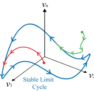
[image:28.612.212.403.271.457.2]

1.1 Basic Setup and Notation

Figure 1.2: Mathematical description of an oscillator as traversing a stable limit cycle in n dimensions. Points in the state space not on the orbit will eventually converge to the limit cycle.

An oscillator is a system that is capable of self-sustaining a periodic signal. Within

the dynamical systems community, oscillators are usually visualized in the state

space (see Figure 1.2) [39]–[43], where they traverse a closed trajectory, a limit cycle, in a fixed amount of time, known as the free-running period of oscillationT0.

Although all observable signals within an electrical oscillator are periodic with this

oscillation periodT0, we will focus on a particular node voltage vosc(t) (or set of

node voltages), which we will call theoscillation voltage.

We are interested in the behavior of this oscillator when it isdisturbedby an external signal of some sort, periodic with a possibly different periodTinj. For our purposes,

(29)

commonly (but not necessarily) the node at which the oscillation voltage is observed.

This setup is depicted conceptually in Figure 1.3.

Figure 1.3: A basic cartoon of the setup and notation underlying the analysis. In the free-running case (i.e.,iinj =0),ξ(t)=0 andϕ(t)=ω0t. Under injection, the phase becomesϕ(t) ≡ω0t+φ(t) ≡ωinjt+θ(t).

In the absence of injection—the free-running scenario—we write the oscillation voltage as

vosc(t)= v0(ω0t),

where theoscillation waveform v0(·)is 2π-periodic, andω0 ≡ 2π/T0 is the

free-running (angular) oscillation frequency. The argument ofv0(·)is thephaseϕof the

oscillator in radians, a quantity which increases by 2πfor each oscillation cycle. On the other hand,v0(·)itself captures the free-runningshapeandsizeof the oscillation

voltage.

In the presence of an external disturbance, two things happen:

1. The oscillator’s phase may no longer increase at a constant rate equal toω0.

2. The oscillation voltage may deviate in size and shape fromv0(·).

Therefore, we write the oscillation voltage in the following form:

vosc(t)= [1+ξ(t)] ·v0[ϕ(t)], (1.1)

(30)

instantaneous oscillation frequencyωoscis defined as the time derivative of the total

phase:

ωosc B dϕ

dt. (1.2)

It should be clear that wheniinj = 0 and the oscillator is free running, ϕ(t) = ω0t

andξ(t) = 0. Denoting the (angular) injection frequency ωinj ≡ 2π/Tinj, it will be

useful to define the additional phasesφ(t)andθ(t)using the following relationship:

ϕ(t) ≡ω0t+φ(t) ≡ωinjt+θ(t). (1.3)

Physically, φ(t)is the phase in excess of free-running (ω0t), and θ(t)is the phase referred to the injection (ωinjt). Table 1.1 reiterates the physical meaning behind

these important quantities. In injection locking and pulling scenarios, it is most

convenient to deal withθas the phase of interest, since we are interested in observing if or how the oscillatorsynchronizesitself to the injection frequencyωinj.

Table 1.1: Oscillator Phase Definitions

ϕ: φ: θ:

Total, Instantaneous Oscillator Phase

Phase in Excess of Free-Running(ω0t)

Phase Referred to the Injection(ωinjt)

At this point, it should be noted from a mathematical standpoint that while the

phase can be accurately represented using a single scalar variable, an oscillator

in d-dimensional state space would require (d −1) other scalars to fully describe its orbital deviations. However, we will see that Eq. (1.1) will prove itself to be sufficient for our purposes, while bringing in the full state-space representation of

the oscillator will clutter up the analysis with a significant amount of mathematical

machinery without contributing much physical insight.

1.2 Definition of Injection Locking and Pulling

The purpose of this study is to characterize the behavior of oscillators under the

influence of a periodic injection. Specifically, we are interested in the scenario

where the oscillator synchronizes itself to the injection and oscillates at the injection

frequency: ωosc = ωinj.1 We then say that the oscillator isinjection locked to the

injection signal. An example of injection locking is shown in Figure 1.4, where an

oscillator which free-runs at f0= 1 GHz is injection locked to a sinusoidal injection

1_{The more general cases of injection-locked frequency division and multiplication will be}

(31)

(a) Top: free-running oscillation voltagev0(ω0t)(blue, dashed curve) and

injection-locked oscillation voltagevosc(t)(red, solid curve). Bottom: injection currentiinj(t).

(b) Magnitude spectra of the free-running and injection-locked oscillation voltages.

Figure 1.4: An example of injection locking. Note that the oscillation voltage is observed at the node being injected into.

at finj =0.8 GHz. Consequently, while the free-running oscillation voltage traverses

10 cycles in the 10 nanosecond interval shown, both the injection current and the

injection-locked oscillation voltage only undergo 8 cycles. Notice how the injection

alters both the shape and the size of the oscillation voltage.

(32)

mathemat-(a) Top: oscillation voltage of an injection-pulled oscillator. Bottom: injection current.

(b) Magnitude spectrum of the injection-pulled oscillation voltage.

Figure 1.5: An example of injection pulling where f0= 1 GHz and finj =0.8 GHz.

ically represented byθbeing constant in time:

Injection Locked ⇐⇒ dθ

dt = 0. (1.4)

The value ofθfor an injection-locked oscillator, which represents the phase differ-ence between the oscillator and the injection, is not arbitrary. For a given oscillator and injection waveform,θ varies with the injection frequency in a specific manner. This relationship is known as thelock characteristic.

(33)

sufficiently close toω0. The range of frequencies that the oscillator can lock to is

known as thelock range. More precisely, the upper/lower lock rangeω±_L is defined as the maximum/minimum value of the frequency deviation ∆ω ≡ ωinj− ω0 for which the oscillator is capable of injection locking. The lock range depends not

only on the oscillator but on the size and shape of the injection waveform as well.

(a) Oscillation voltage and injection current.

(b) Threshold-crossing difference normalized to the injection period.

Figure 1.6: Zooming into a single “beat” for the injection-pulled oscillator of Figure 1.5.

If the injection fails to lock the oscillator because it is outside of the lock range,

then dθ/dt _, 0 and we instead say that the oscillator is injection pulled by the

injection signal. An example of injection pulling is depicted in Figure 1.5, obtained

(34)

injection-locked example of Figure 1.4. The frequency of the “beats” which appear in the

time-domain plot of the oscillation voltage is equal to the distance between the adjacent tones in the frequency-domain spectrum. A closer look at what happens during

one of these low-frequency beats is shown in Figure 1.6. Essentially, the injection

“attempts” to lock the oscillator, but is unable to effect a sufficiently large change

in the oscillation frequency, causing the oscillator to eventually “slip” by an entire

cycle compared to the injection signal. One way of visualizing this is to compare the

threshold crossing times of the oscillator and the injection. Specifically, consider the

difference between the falling-edge 0.5 V-crossing times of the oscillation voltage and the falling-edge zero-crossing times of the injection, normalized toTinj. This

parameter increases (or decreases) by 1 whenever the oscillator retards (or advances) by a single cycle relative to the injection. Figure 1.6b plots this parameter as a

function of the number of elapsed cycles for the window under consideration and

compares the result against the injection-locked and free-running scenarios. As

we can see, an injection-locked oscillator features a constant threshold-crossing

difference over all cycles, whereas the threshold-crossing difference must grow by

a fixed amount per cycle for a free-running oscillator (at a different frequency).

On the other hand, for an injection-pulled oscillator, while the injection “tries” to

keep this threshold-crossing difference constant, it eventually fails and the oscillator

“runs off on its own” by an entire cycle. In light of this repeated behavior, one might suspect that the oscillation voltage of an injection-pulled oscillator is periodic

with this (lower) beat frequency ωb. Unfortunately, this is not correct unless the injection frequencyωinjis amultipleofωb, which is not true in general. Therefore,

we surmise that the periodicity of the oscillator is corrupted by injection pulling.

1.3 Organization of Thesis

The rest of this thesis is organized as follows. Chapter 2 puts this work into context

by reviewing existing injection locking and pulling models. A distinction is made

between mathematical macromodeling approaches, which our theory falls under, and

physically-based behavioral analyses. Chapter 3 conducts a thought experiment that

examines the effect an impulse train has on an ideal LC oscillator. The understanding

gleaned from this thought experiment will motivate the development of our model from a conceptual standpoint.

Chapter 4 develops, from first principles, a time-synchronous theory of oscillators

that are subjected to a periodic external perturbation. We demonstrate how the

(35)

injection locking. Chapter 5 augments the theory for the specific case of the LC

oscillator by accounting for the oscillation amplitude, resulting in a model which is applicable for large injections. Novel insights into how different types of LC

oscillators behave, which are uniquely captured by this model, are also provided.

Chapter 6 generalizes the framework to allow for an arbitrary rational relationship

between the injection and oscillation frequencies under lock.

Chapter 7 focuses on an analysis of the transient behavior of periodically disturbed

oscillators. Issues such as mode stability, the pull-in process, and the dynamics of

injection pulling are covered. A theoretical treatment of the effect of astochastic

disturbance, which illuminates the elementary connection between phase noise and

injection locking, is also performed. Chapter 8 explores design insights which arise

from the developed framework. Specifically, several ways of enhancing an

oscil-lator’s lock range are introduced and demonstrated. Chapter 9 uses the techniques

discussed in Chapter 8 to implement a low-power injection-locked prescaler for

frequency synthesis applications.

Chapter 10 takes an alternative, physical viewpoint of injection locking and carries

out a phasor-based analysis of sinusoidal injection locking in LC and ring oscillators. Future research directions are suggested in Chapter 11, and other unrelated works

(36)

C h a p t e r 2

EXISTING MODELS

“All models are wrong, but some are useful.”

George Edward Pelham Box, 1976

Injection locking and pulling of electrical oscillators has been studied extensively

for at least the past century [44]–[85]. In this chapter, we give a brief overview

of the existing models in the literature which are used more prominently in the

electronics community. In general, any analysis technique can be categorized as

either abehavioral modelor amathematical macromodel.

2.1 Behavioral Models

Behavioral approaches start with aphysicalmodel of the oscillator under injection, such as a circuit model comprising resistors, capacitors, inductors, idealized

non-linear elements, and the injection source(s). Known analysis techniques for this

physical model (e.g., KCL/KVL, Ohm’s Law, phasors) are then used to study the system, leading to conclusions about aspects of the system’s behavior that we seek

to understand. Due to their physically-based nature, such approaches tend to provide

intuition more directly. But their utility is limited because the analysis is restricted

to a particular oscillator topology (e.g., LC, ring, or relaxation), and their predictive

power is constrained by the accuracy of the model itself. The analysis presented in

Chapter 10 of this thesis is a behavioral model.

Adler’s Equation

Both experimental and theoretical work on the synchronization of electrical

oscil-lators have been conducted as early as the 1920’s [44]–[46]. However, perhaps the

most well-known behavioral model for injection locking is Adler’s equation,

devel-oped by Robert Adler in 1946 [47]. Adler’s equation describes the phase of an LC oscillator under the influence of a weak sinusoidal injection close to the free-running

oscillation frequency.

We present a simplified derivation here. Consider the ideal LC oscillator shown

in Figure 2.1. The loss of the LC tank, represented by the parallel resistance RP,

(37)

fundamental component is in phase withvosc(t)and has an amplitude of Iosc. The

oscillator free-runs at the LC tank’s resonant frequency

ω0=

1

√

LC. (2.1)

The current consumed by the resistance is supplied by the oscillator current Iosc,

leading to a sinusoidal oscillation amplitude of

Vosc = IoscRP. (2.2)

Figure 2.1: Schematic of the basic LC oscillator under injection used in the deriva-tion of Adler’s equaderiva-tion.

Suppose a weak sinusoidal currentiinj(t)in the close vicinity ofω0 is injected into the oscillator as shown. Utilizing complex exponential notation to simplify the

subsequent algebra, we express the injection current as

iinj(t)= Iinjejωinjt, (2.3)

where the injection amplitude issmallin the sense thatIinj Iosc, and the injection

frequency is near the free-running frequency in the sense thatωinj−ω0

ω₀. We

adopt the usual convention from Eq. (1.3) of expressing the phase of the oscillation

voltage asωinjt+θ(t), where the objective of this analysis is to study the behavior of θ, the phase difference between the oscillator and the injection. Because the injection is weak compared to the oscillator current, its impact on the resistor currentiR is negligible, leaving the oscillation amplitudeVosc = IoscRP unchanged. Therefore,

we write the oscillation voltage as

vosc=Voscej(ωinjt+θ), (2.4)

and we instead focus on how the injection influences the LC tank by writing KCL

for the remaining currents:

iinj =iC+iL

=⇒ diinj dt =C

d2vosc

dt2 +

vosc L .

(38)

The intuition here is that the reactive current drawn by the LC tank when the

oscillator operates away from resonance must be supplied by the injection current. Substituting for the injection current and the oscillation voltage, we get

jωinjIinjejωinjt = ( C " jd 2_θ dt2 −

ωinj+ dθ dt

2# + 1

L )

IoscRPej(ωinjt+θ). _(2.6)

Multiplying through bye−j(ωinjt+θ)_{and taking the real part, we get}₁

−

ωinj+ dθ dt

2

+ω02= Iinj Iosc

ω0ωinj

Q sinθ, (2.7)

where we used the tank’s quality factor

Q = RP ω0L =

RPω0C. (2.8)

To simplify the left-hand-side, we use the fact thatω_inj−ω₀

ω₀to approximate ω02−ωinj2≈ 2ωinj(ω0−ωinj), and we assume thatθvariesslowlyin comparison to

the injection: dθ dt

ω_inj. (2.9)

With these approximations, we obtain

2ωinj

ω0−ωinj− dθ dt

= Iinj Iosc

ω0ωinj

Q sinθ. (2.10)

Rearranging, we arrive at Adler’s equation:

dθ

dt = ω0−ωinj− ω0

2Q Iinj Iosc

sinθ. (2.11)

Sinceθis constant under lock, the maximum frequency deviation that the oscillator can lock to, known as the lock range, is given by

ωL = ω0

2Q Iinj

Iosc. (2.12)

One of the key insights resulting from Adler’s equation is that the lock range

increases with the relative injection strength Iinj/Iosc but varies inversely with the tank’s quality factorQ.

Recall the fundamental assumptions underlying this derivation:

1_{Obviously, both the real and imaginary parts need to be satisfied. In a more detailed analysis}

(39)

1. The injection is much weaker than the oscillator: Iinj Iosc.

2. The frequency deviation is small: ωinj−ω0

ω₀.

3. The oscillator’s phase varies slowly relative to the injection: |θ0(t)| ω_inj.

In light of Adler’s equation, the third assumption is implied by the first two. We will

challenge the first two conditions in this thesis.

Because of the accurate conclusions about the lock range, the pull-in process, and

the presence of “beats” in an unlocked oscillator that Adler’s equation is able to

predict, it has formed the basis for numerous other approaches to understanding

injection locking and pulling in electrical oscillators.

Related Works

Many have built upon Adler’s work over the years. Notable examples include generalizing the treatment to non-triode oscillator topologies (Huntoon and Weiss,

1947) [48], modifying the equation for the lock range to account for large injection

currents (Paciorek, 1965) [49], focusing on the unlocked behavior of

injection-pulled oscillators (Stover, 1966; Armand, 1969) [50], [51], extension of the analysis

to microwave oscillators with distributed elements (Kurokawa, 1973) [52], [53],

and coming up with alternative derivations of Adler’s equation as well as applying

Adler’s equation in different settings to glean new insights (Razavi, 2004) [38].

Even recent works which focus on significantly more complicated scenarios, such

as mutual pulling between VCOs residing in different PLLs [86], often use Adler’s equation as a starting point for their analysis.

Mirzaei’s Generalized Adler’s Equation

The most powerful generalization of Adler’s equation to date was proposed by

Mirzaei et al. in 2006 [59], where they use KCL and KVL to analyze the LC oscillator without assuming a weak injection signal. Consequently, the result of

their analysis, which they call “Generalized Adler’s equation,” accounts for how the

injection can influence theamplitude of oscillation—not just the phase. In doing so, the termIoscin Adler’s equation Eq. (2.11) is replaced with Iosc+Iinjcosθ:

dθ

dt = ω0−ωinj− ω0

2Q

Iinjsinθ Iosc+Iinjcosθ

. (2.13)

They then use this equation to conduct a rather thorough analysis of the quadrature

(40)

modern high-frequency systems. The lock range associated with this more general

equation can be shown to be [38], [49], [59]

ωL = ω0

2Q Iinj Iosc

1

s

1− Iinj 2

Iosc2

. (2.14)

In this thesis, we will demonstrate how both the time-synchronous model developed

in Chapters 4 and 5 as well as our phasor-based analysis presented in Chapter 10

analytically reduce to Adler’s equation and its generalization by Mirzaeiet al.

Models for Ring Oscillators

Figure 2.2: A nonlinear model of the ring oscillator often used for injection locking and pulling applications.

The most conspicuous limitation associated with Adler’s equation and its surround-ing body of work is, of course, the fact that the analysis pertains only to LC

oscillators. Consequently a variety of behavioral approaches for modeling

injec-tion locking in ring oscillators have also been developed.2 The approach which

has gained the most traction in recent years models each stage of the ring as an

RC-delay cell driven by an idealized, nonlinear transconductor [10], [60]–[65], as

shown in Figure 2.2. In particular, this behavioral model allows for each node of

the ring oscillator to be injected into, a technique which can widen the lock range

significantly (see Section 6.7).

Among these approaches, several have stood out. The model proposed by Gangasani

and Kinget [61], [62] is slightly more general in that it allows for an arbitrary delay 2_{The other type of non-LC electrical oscillator, the relaxation oscillator, has received much less}

(41)

dynamic (the “d-∆relationship”) for each stage of the ring. On the more practical

side, the analyses carried out by by Chienet al.[63] and Mirzaei et al.[10], [60] have led to the design of wideband CMOS ring-oscillator-based injection-locked

frequency dividers.

2.2 Mathematical Macromodels

In contrast to behavioral or physically-based approaches, macromodeling techniques

start with a collection of fundamental mathematical properties of the system under

study (e.g., linearity, time-invariance, memory, causality). An abstract, general

description of an arbitrary system that satisfies these properties is then formulated,

allowing for certainparameters3of interest to be identified (e.g., impulse response, transfer function, scattering matrix, Fourier series coefficients). These parameters

are then calculated analytically, simulated, or even measured for the actual system of interest (i.e., the oscillator) and then used to make conclusions about the physical

properties of the system that we want to figure out.

The key to successful macromodeling lies in the choice of these parameters—they

need to be sufficiently easy to ascertain, but they also need to capture enough

information about the system’s behavior to be useful. In effect, these parameters

serve as anintermediary between the fundamental physics governing the system’s operation and the system’s characteristics that we are actually interested in, as it

would be too difficult or computationally intractable to derive the latter from the former directly. As an example, it would not be feasible or necessary to perform

a full-blown, brute-force analysis of the current through every branch and voltage

at every node of an oscillator just to derive its phase noise or synchronization

properties.

Such approaches tend to be very general in their applicability, but due to their abstract

nature, care must be taken when interpreting their results to ensure that they are both

physically meaningful and practically insightful. An exemplar of a mathematical

macromodel which simultaneously possesses tremendous predictive power while being intuitive to understand is Hajimiri and Lee’s oscillator phase noise model

[87]–[90]. The core parameter at the heart of their model is a periodically

time-varying impulse response of the oscillator’s phase with respect to noise, embodied

in a parameter they named the Impulse Sensitivity Function (ISF) Γ(x). The ISF will be discussed extensively in Chapter 4. The model developed in the bulk of

3_{Note that a “parameter” in this context could be a function, a scalar or matrix variable, a}