Overview of Important Algorithms to mine
Frequent Patterns from Uncertain Data
Vani Bhogadhi
1, Dr. M. B. Chandak
21Student (M.Tech), Department of Computer Science and Engineering, RCOEM, Nagpur, Maharashtra, India 2 Head, Department of Computer Science and Engineering, RCOEM, Nagpur, Maharashtra, India
Abstract— In this paper, we focus on some of the important algorithms used in mining frequent patterns from uncertain data. The algorithms discussed are UF-growth, CUF-UF-growth, PUF-UF-growth, tubeS-UF-growth, tubeP-growth. Uncertainty in data is caused by factors like data
randomness, data incompleteness, etc. In some
circumstances, users are interested in only some of the frequent patterns instead of all. The user can express his interest in terms of constraints and push them into the mining process as a result, the search space is reduced which is termed as constrained mining. Finally, big data has brought tools for the problem of frequent pattern mining of uncertain data.
Keywords— big data, constrained mining, data randomness, Frequent pattern mining, uncertain data.
I. INTRODUCTION 1.1 Frequent Pattern Mining
Finding frequent patterns plays an essential role in association rule mining, classification, clustering, and other data mining tasks. Frequent pattern mining [17, 19] was first proposed by Agrawal et al.[17] for market basket analysis in the form of association rule mining. It analyses customer buying habits by finding associations between the different items that customers place in their “shopping baskets”. Let I = {i1, i2, ... , in} be a set of all items. A k-itemset α, which consists of k items from I, is frequent if α occurs in a transaction database D no lower than θ|D| times, where θ is a user-specified minimum support threshold (called min_sup), and |D| is the total number of transactions in D.
1.2 Uncertainty in Data
How much faith can or should be put in the Social media data like Tweets, Facebook posts, etc. Correlation of the data with persons, items, locations, associations, etc can somewhat reduce uncertainty but cannot completely eliminate it. Sure, this data can be used as a count toward sentiment, but cannot be used as a count for total sales and report on that. Due to measurement errors, but also sensor malfunctions, approximation errors, sampling errors, etc sensor data is highly uncertain as well. Due to the sheer velocity of some data (like stock trades, or
machine/sensor generated events), time cannot be spent to “cleanse” it and get rid of the uncertainty, so data must be processed as is i.e. understanding the uncertainty in the data. Nowadays, as multi-structured data is being brought together, it is nearly impossible to determine the origin of the data and correlate fields.
Data can be obsolete (e.g., when a dynamic database is not up-to-date), data may originate from unreliable sources (such as crowd-sourcing), the volume of the dataset may be too small to answer questions reliably, or Data may be blurred to prevent privacy threats and to protect user anonymity. The challenge in handling uncertain data is to obtain reliable results despite the presence of uncertainty.
1.3 Probabilistic Model for Uncertain Data
Users may not be certain about the presence or absence of an item x in a transaction ti in a probabilistic dataset D of
uncertain data [20]. Users may suspect, but cannot guarantee, that x is present in ti. The uncertainty of such
suspicion can be expressed in terms of existential probability P(x, ti), which indicates the likelihood of x
being present in ti in D. The existential probability P(x, ti)
ranges from a positive value close to 0 (indicating that x has an insignificantly low chance to be present in D) to a value of 1 (indicating that x is definitely present). With this notion, each item in any transaction in traditional databases of precise data (e.g., shopper market basket data) can be viewed as an item with a 100 % likelihood of being present in such a transaction.
1.4 Objectives of the Paper
www.ijaems.com Page | 324 II. FREQUENT PATTERN MINING OF
UNCERTAIN DATA
Uncertain frequent pattern mining from a probabilistic dataset D of uncertain data is to find every pattern X having expSup(X,D) ≥ minsup. Such a pattern X is called an expected support-based frequent pattern or just frequent pattern
Finding frequent patterns from uncertain data started with candidate generate-and-test paradigm and now replaced with tree-based mining due to its advantages.
2.1 Uncertain Frequent Pattern Mining using candidate generate-and-test paradigm (U-Apriori)
Chui et al. proposed U-Apriori algorithm [1], a modification of Apriori algorithm [17] that mines frequent patterns from uncertain data. U-Apriori algorithm uses candidate generate-and-test paradigm in a breadth first bottom-up fashion.
U-Apriori Algorithm:
Step 1: computes the expected support of all domain items. Those items with expected supports ≥ minsup become every frequent pattern consisting of one item. Step 2: the algorithm repeatedly applies the candidate generateandtest process to generate candidate (k+1) -itemsets from frequent k--itemsets and test if they are frequent (k+1)-itemsets.
The algorithm’s efficiency can be improved by including the LGS-trimming strategy (local trimming, global pruning, and single-pass patch up) [1]. This strategy trims away every item with an existential probability below the user-specified trimming threshold (which is local to each item) from the original probabilistic dataset D of uncertain data and then mines frequent patterns from the resulting trimmed dataset DTrim. On the one hand, if a
pattern X is frequent in DTrim, then X must be frequent in
D.
U-Apriori algorithm suffers from the following problems:
• there is an overhead in creating DTrim • only a subset of all the frequent
• patterns can be mined from DTrim and there is
overhead to patch up
• the efficiency of the algorithm is sensitive to the percentage of items having low existential probabilities
• it is not easy to find an appropriate value for the user-specified trimming threshold
• there are multiple scans involved
2.2 Uncertain Frequent Pattern Mining using Tree Structures
The candidate generate-and-test based mining algorithms (e.g., the U-Apriori algorithm) use a levelwise bottom-up breadth-first mining technique to find frequent patterns from uncertain data. As an alternative to Apriori-based,
tree-based mining avoids generating many candidates. Tree-based algorithms use a depth-first divide-and-conquer approach to mine frequent patterns from a tree structure that captures the contents of the probabilistic dataset.
The UF-growth is a tree based algorithm for mining uncertain data to find the frequent itemsets proposed by Leung et.al. [10]. The two main steps in this algorithm are
• the construction of UF-trees
• mining of frequent patterns from UF-trees. While construction of the UF-tree each node captures an item, its expected support and the number of occurrence of such expected support for such an item. The UF-growth algorithm constructs the UF-tree as follows: It scans the database once and accumulates the expected support of each item. Hence, it’s all frequent items (i.e., items having expected support ≥ minsup). It sorts these frequent items in descending order of accumulated expected support. The algorithm then scans the database the second time and inserts each transaction into the UF-tree.
2.3 CUF Tree Structure
Leung and Tanbeer[2] proposed the capped uncertain frequent pattern tree (CUF-tree) structure, which uses the tree structure to represent the items of the transaction and also extracts the frequent patterns from the tree. Here the CUF-tree is constructed by considering an upper bound of existential probability for each transaction which is called as the cap of the transaction existential probability. Definition: The transaction cap of a transaction ti,
denoted as Pcap(ti), is defined as the product of the two
highest existential probability values of items within ti.
Let h=| ti | represent the length of ti, M1 = maxqє[1,h]P(xq, ti)
and M2 = maxrє[1,h],r≠q P(xr, ti).
M1 × M2 if h>1
PCap(ti) = P(x1, ti) if h=1 (1)
Where the PCap(ti) provides users with an upper bound
of existential probability values of all possible k-itemsets (where k > 1) in each transaction.
The cap of expected support of an itemset X, denoted as expSupCap(X), is defined as the sum of all transaction caps of ti in which X occurs, expSup
Cap
(X)=∑i=1 n
PCap(ti)│X⊆ti), n=|DB|.
CUF Tree Construction Algorithm:
The CUF-tree is constructed in two database scans.
• In the first scan of the database, the expected support of each domain item is calculated, thereby removing infrequent items, and then all frequent items are sorted in descending order of their total expected support.
• In the second scan of the database, CUF-tree is constructed and the transaction caps are calculated at the same time.
• Items of the transaction are inserted into the CUF-tree according to the sorted list order, and the transaction cap value is added to each node according to the sorted list order.
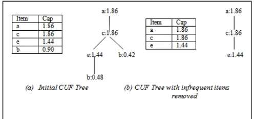
Consider Table 1 with four transactions, and let the minsup be 1.0. The above algorithm computes the expected support of each item as {a: 2.3, b:1.4, c:2.2,d:0.9, e:1.8}, removes infrequent items from the list, and arranges the remaining items in sorted order results in item-list {a:2.3, c:2.2, e:1.8, b:1.4}. Then in the second scan of the database, transaction cap of each transaction are calculated and CUF Tree is also constructed. Only frequent items are considered while calculating the transaction cap which results in the tighter upper bound for the construction of the CUF Tree and eventually generates less number of false positives. The initial and the final item caps and their corresponding CUF-trees after removing the infrequent items are shown in the Figure 1.
The CUF-growth algorithm is responsible for constructing the projected databases and mining frequent patterns from uncertain data. It scans the database three times to extract the frequent patterns. The algorithm calculates the transaction caps in its first scan and builds the CUF-tree during its second scan. The tree stores the
item and the transaction caps, which act as the upper bounds to the expected support of frequent k-itemsets (for k≥2). The last step in the algorithm during the second scan is to discover all possible frequent patterns by extracting suitable tree paths from subsequent projected databases. There may be some infrequent patterns (false positives) so the algorithm again scans the dataset for the third time to check whether all the frequent patterns retrieved during the second scan are truly frequent patterns or not and trims the false positives.
Fig.1: CUF-Tree
2.4 PUF Tree Structure
Leung and Tanbeer[3] proposed the PUF-tree which is constructed by considering an upper bound of existential probability value for each item when generating a k-itemset (where k > 1). We call the upper bound of an item xr in a transaction ti the (prefixed) item cap of xr in ti, as
defined below.
Definition: The (prefixed) item cap ICap(xr, ti) of an item xr
in a transaction ti = {x1, . . . , xr, . . . , xh}, where 1 ≤ r ≤ h,
is defined as the product of P(xr, ti) and the highest
existential probability value M of items from x1 to xr−1 in
ti (i.e., in the proper prefix of xr in ti):
P(xr, ti)×M if h>1, where M= max1≤q≤r- 1
P(xq, ti)
ICap(xr,ti)= P(x1, ti) if h=1 (2)
The cap of expected support expSupCap(X) of a pattern X= {x1, . . . , xm} (where m > 1) is defined as the sum
(over all n transactions in a DB) of all item caps of xm in
all the transactions that contain X: expSupCap(X)=
∑i=1n{ICap(xm ,ti)|X⊆ti)
TABLE II. A TRANSACTION DATABASE USING MINSUP=0.5
TID Contents Contents(after 1st scan) P
Cap
t1 {a:0.5, b:0.8, c:0.5, e:0.6}
{a:0.5, b:0.8, c:0.5,
e:0.6} 0.48 t2 {a:0.7, b:0.6, c:0.6,
d:0.7} {a:0.7, b:0.6, c:0.6} 0.42 t3 {a:0.3, c:0.8, e:0.5} {a:0.3, c:0.8, e:0.5} 0.40 t4 {a:0.8, c:0.3, d:0.2,
www.ijaems.com Page | 326
PUF Tree is constructed as shown below:
In the first scan of the database, it finds distinct frequent items in DB and constructs an I-list to store only frequent items in some consistent order (e.g. canonical order) to facilitate tree construction.
• The PUF-tree is constructed with the second database scan in a fashion similar to that of the FP-tree [4].
• Before inserting an item into the tree, its item cap is calculated and then inserted into the tree according to the I-list order.
If that node already exists in the path, we update its item cap by adding the computed item cap to the existing item cap. Otherwise, we create a new node with this item cap value.
PUF trees which includes all the items of all transactions and after removing infrequent items are shown in the following Figure 2.
Fig.2. PUF-Tree
The PUF-growth algorithm takes three scans of the probabilistic dataset of uncertain data to mine frequent patterns.
• In the first scan, PUF-growth computes the prefixed item caps.
• During the second scan, PUF growth builds a PUF-tree and stores the item and its corresponding prefixed item cap.
• By the end of the second scan PUF-growth finds all the frequent patterns by forming the PUF-trees for subsequent projected databases.
• Finally in the third scan it verifies each frequent pattern is truly frequent by pruning the false positives.
CUF and PUF-growth algorithms construct tree structures with the help of item caps where the size of the trees are very small when compared with the UF-tree. PUF-growth is faster than CUF-growth. We can obtain a compact tree structure by further reducing the upper bound on expected support results in a tree structures, called tube-trees namely tubeS and tubeP-trees [23].
2.5 TubeS Tree Structure
Leung and Tanbeer [23] proposed the TubeS-tree which is constructed by considering the second highest existential probability value in the proper prefix for each transaction generating a k-itemset (where k > 1).
Each path in the tree represents a transaction and in turn each node in the tree maintains (i) an item xr in in a
transaction ti = {x1, . . . , xr, . . . , xh}, (ii) its item cap
ICap(xr,ti), and (iii) the second highest probability M1(xr,ti)
in the proper prefix {x1, . . . , xr-1}⊆ ti. The tightened
upper bound to expected support on a second highest existential probability (tubeS) for X={x1. . . xr, . . . , xh}⊆
ti is calculated as :
ICap (X, ti) if k ≤ 2
tubeS (X, ti)= ICap (X, ti) × πi=1 k-2 M1(xr, ti) if k ≥ 3 (3)
where M1(xr,ti) is the second highest existential
probability value among all r-1 items in the proper prefix {x1, . . . , xr-1}⊆ ti and ICap(xr,ti) value is taken from
Equation(2).
2.6 TubeP Tree Structure
Each node in the tree maintains (i) an item xr in in a
transaction ti = {x1, . . . , xr, . . . , xh}, (ii) its item cap
ICap(xr,ti), and (iii) its existential probability P(xr, ti). With
this information, another tightened upper bound to expected support based on existential probabilities of prefix item (tubeP) for X={x1. . . xr, . . . , xh}⊆ ti is
calculated as
ICap (X, ti) if k ≤ 2
tubeP (X, ti)= I Cap
(X, ti) × πi=1 k-2
P(xr, ti) if k ≥ 3 (4)
where P(xr, ti) is the existential probability of xr € ti
The second highest existential probability value M1(xr,ti)
and the P(xr, ti) value that are used in both tubeS and
tubeP-growth guarantees not to generate high cardinality candidates due to their expected support caps being closer to the actual expected support.
TID Transactions
Sorted transactions with infrequent items removed t1 {a:0.3, b:0.1, c:0.9,
f:0.6} {a:0.3, c:0.9, f:0.6} t2 {a:0.6, c:0.8, e:0.4} {a:0.6, c:0.8, e:0.4} t3 {a:0.4, d:0.4, e:0.5,
f:0.4}
{a:0.4, d:0.4, f:0.4, e:0.5}
t4 {a:0.8, b:0.3, d:0.1,
III. CONSTRAINED UNCERTAIN FREQUENT PATTERN MINING
The CUF-growth and PUF-growth algorithms are useful in finding all the frequent patterns from probabilistic datasets of uncertain data in many situations. There are many real-life situations in which the user is interested in only some frequent patterns. Finding all frequent patterns would then be redundant and waste lots of computation. This leads to constrained mining [5, 6, 7, 8, 9] that aims in finding only those frequent patterns that are interesting to the user. In response, Leung et al. [10, 11] extended the UF-growth algorithm to mine probabilistic datasets of uncertain data for frequent patterns that satisfy user-specified constraints resulting algorithm, called U-FPS [10] which effectively find constrained frequent patterns from uncertain data.
Users typically employ their knowledge of the application or data to specify rule constraints for the mining task. In general, an efficient frequent pattern mining processor can prune its search space during mining in two major ways: pruning pattern search space and pruning data search space. Based on how a constraint may interact with the pattern mining process, there are five categories of pattern mining constraints antimonotonic, monotonic, succinct, convertible and inconvertible.
Antimonotonic: If an itemset does not satisfy the rule constraint, none of its supersets can satisfy the constraint. Monotonic: When an item set S satisfies the constraint, so does any of its superset.
Succinct Constraints. This constraint enumerates all and only those sets that are guaranteed to satisfy the constraint.
Once the UF-tree is constructed, the U-FPS(SAM)[10] algorithm recursively mines frequent patterns that satisfy SAM constraints from this tree in a similar fashion as in the FP-growth[4] algorithm. The U-FPS effectively mines from uncertain data all and only those frequent patterns that satisfy the user-specified SAM constraint.
IV. UNCERTAIN FREQUENT PATTERN MINING FROM BIG DATA
"Big Data"[12] is a term used to describe a massive volume of diverse data, both structured and unstructured, that is so large and fast-moving that it’s difficult or impossible to process using traditional databases and software technology. In most enterprise scenarios, the data is too enormous, streaming by too quickly at unpredictable and variable speeds, and exceeds current processing capacity.
In 2012, Gartner revised and gave a more detailed definition [21, 22] as: Big Data are volume, high-velocity, and/or high-variety information assets that require new forms of processing to enable enhanced
decision making, insight discovery and process optimization”. More generally, a data set can be called Big Data if it is formidable to perform capture, curation, analysis and visualization on it at the current technologies MapReduce[14] is a software framework which facilitates the user to write applications to process huge amounts of data, in parallel, on large clusters of commodity hardware in a reliable manner. MapReduce is a processing technique and a program model for distributed computing based on java. The MapReduce algorithm contains two important tasks, namely Map and Reduce. Map takes a set of data and converts it into another set of data, where individual elements are broken down into tuples (key/value pairs). Secondly, reduce task, which takes the output from a map as an input and combines those data tuples into a smaller set of tuples. The major advantage of MapReduce is that it is easy to scale data processing over multiple computing nodes. Once we write an application in the MapReduce form, scaling the application to run over hundreds, thousands, or even tens of thousands of machines in a cluster is merely a configuration change. This simple scalability is what has attracted many programmers to use the MapReduce model.
To mine frequent patterns from Big probabilistic datasets of uncertain data, Leung and Hayduk [13] proposed the MR-growth algorithm. The algorithm uses MapReduce by applying two sets of the “map” and “reduce” functions—in a pattern growth environment. Specifically, the master node reads and divides a probabilistic dataset D of uncertain data into partitions, and then assigns them to different worker nodes. During the first set of map phase each worker node emits the item(x) and the probability associated with that item and transaction in which the item is present (P(x, tj). These <x, P(x, tj) )>
pairs in the list (i.e., intermediate results) are shuffled and sorted (e.g., grouped by x). Each worker node then executes the “reduce” function, which (i) “reduces”—by summing—all the P(x, tj) values for each item x so as to
compute its expected support expSup({x},D) and (ii) outputs <{x}, expSup({x},D)> (representing a frequent singleton {x} and its expected support) if expSup({x},D)
≥ minsup.
www.ijaems.com Page | 328
using the two sets of “map” and “reduce” functions, the MRgrowth algorithm finds
• all frequent one-itemsets with their expected support
• then builds appropriate projected databases using FP-trees, CUF-trees or PUF-trees to find all frequent k-itemsets (for k ≥ 2) with their expected support.
V. CONCLUSION
Many candidate sets will be generated and tested for their frequency in U-Apriori algorithm. This generate-and-test procedure is completely avoided in tree based frequent pattern mining algorithms. Larger tree sizes in UF-tree are reduced in subsequent algorithms using Caps (Limits). In PUF-growth prefixed item caps are used to reduce false positives in comparison to usage of transaction caps in CUF-growth. tubeS-growth and tubeP-growth ensure non-generation of high cardinality candidates and thereby improve run-time performance. The above mentioned algorithms generates all the possible frequent patterns but if the user is interested in only some part of the frequent patterns then constrained frequent pattern mining is used. U-FPS algorithm enables the user to push the constraints into the mining process. MR-growth algorithm is used to mine the frequent patterns from Big Data for analytics. In the context of Bigdata, Uncertain frequent pattern search space can be greatly reduced using constrained mining.
REFERENCES
[1] Chui, C.-K., Kao, B., & Hung, E. 2007, “Mining frequent itemsets from uncertain data,” in Proceedings of the PAKDD 2007, pp 47–58. Springer.
[2] Leung, C.K.-S., & Tanbeer, S.K. 2012, “Fast tree-based mining of frequent itemsets from uncertain data”, in Proceedings of the DASFAA 2012, Part I, pages 272–287. Springer.
[3] Leung, C.K.-S., & Tanbeer, S.K. 2013, “PUF-tree: a compact tree structure for frequent pattern mining of uncertain data,” in Proceedings of the PAKDD 2013, Part I, pages 13–25. Springer.
[4] Chi, Y., Muntz, R.R., Nijssen, S., Kok, J.N, “Frequent subtree mining- an overview,” in Proceedings of the PAKDD 2013. 66(1-2), 161-198 (2004)
[5] Cuzzocrea, A., Leung, C.K.-S., & MacKinnon, R.K. 2014, Mining constrained frequent itemsets from distributed uncertain data”, in Future Generation Computer Systems. Elsevier.
[6] Lakshmanan, L.V.S., Leung, C.K.-S., & Ng, R.T. 2003, “Efficient dynamic mining of constrained frequent sets,” in ACM Transactions on Database Systems (TODS), 28(4), pp 337–389.
[7] Leung, C.K.-S. 2009, “Frequent itemset mining with constraints,” in Encyclopedia of Database Systems, pp 1179–1183. Springer.
[8] Leung, C.K.-S., & Brajczuk, D.A. 2009, “Mining uncertain data for constrained frequent sets,” in Proceedings of the IDEAS 2009, pp 109–120. ACM. [9] Leung, C.K.-S., & Brajczuk, D.A. 2010, “uCFS2: an enhanced system that mines uncertain data for constrained frequent sets,” in Proceedings of the IDEAS 2010, pp 32–37. ACM.
[10] Leung, C.K.-S., & Brajczuk, D.A. 2009, “ Efficient algorithms for the mining of constrained frequent patterns from uncertain data,” in ACM SIGKDD Explorations, 11(2), pp 123–130.
[11] Leung, C.K.-S., Hao, B., & Brajczuk, D.A. 2010, “Mining uncertain data for frequent itemsets that satisfy aggregate constraints,” in Proceedings of the ACM SAC 2010, pp 1034–1038
[12] Madden, S. 2012, “From databases to big data,” in IEEE Internet Computing, 16(3), pp 4–6.
[13] Leung, C.K.-S.,&Hayduk,Y. 2013, “Mining frequent patterns from uncertain data with MapReduce for Big Data analytics,” in Proceedings of the DASFAA 2013, Part I, pp 440–455. Springer. [14] http://www.tutorialspoint.com/hadoop/hadoop_mapr
educe.htm
[15] Carson Kai-Sang Leung, Mark Anthony F. Mateo, and Dale A.Brajczuk, “A Tree-Based Approach for Frequent Pattern Mining from uncertain Data”, T. Washio et al. (Eds.): PAKDD 2008, LNAI 5012, pp. 653–661, 2008
[16] Mohammad Mudassar Khan, Anand Rajavat , “An Efficient Algorithm for Extracting Frequent Item Sets from a Data Set”. In Proceedings of the International Journal of Advanced Research in Computer Science and Software Engineering, pp 1373-1375.
[17] R. Agrawal and R. Srikant,”Fast Algorithms for Mining Association Rules in Large Databases,” in Journal of Computer Science and Technology, vol. 15, pp. 487-499,1994
[18] Lukoianova, T., & Rubin, V. (2014), “Veracity Roadmap: Is Big Data Objective, Truthful and Credible?,” in Advances In Classification Research Online, 24(1). doi:10.7152/acro.v24i1.14671 [19] Agrawal, R., Imielinski, T., & Swami, A, “Mining
association rules between sets of items in large databases,” in Proceedings of the ACM SIGMOD 1993, pp 207–216.
Engineering, 29(1), pp 17–24. IEEE Computer Society.
[21] http://www.gartner.com/resId=2057415
[22] L.W.M. Wienhofen, B.M. Mathisen, D. Roman, “Empirical Big Data Research: A Systematic Literature Mapping,” http://arxiv.org/pdf/1509.03045.pdf.
![Was ist Männergesundheit? Eine Definition [What is Men's Health? A definition]](data:image/gif;base64,R0lGODlhAQABAIAAAP///wAAACH5BAEAAAAALAAAAAABAAEAAAICRAEAOw==)