Data Driven Computing
Thesis by Trenton Kirchdoerfer
In Partial Fulfillment of the Requirements for the Degree of
Doctor of Philosophy
California Institute of Technology Pasadena, California
2018
Acknowledgments
First thanks go to my adviser Michael Ortiz, who provided guidance, showed patience and shared experience all to my benefit. His demonstrated research strategies have embodied a fundamental way of examining problems I will forever associate with him, Caltech and the advancement of science. I am extremely grateful to have been able to work with so able a mentor. I am also thankful to the many members of the Ortiz group, including Lydia and Marta, with whom I have frequently discussed life and work. In this vein special thanks are owed to Amuthan, who opened his door to my questions and requests for aide too many times to count. I remain indebted to the many other friends and classmates who were pivital in helping me navigate the difficulties of graduate life. I also recieved a great deal of guidance and advise from my coworkers and managers at the Southwest Research Institute, which provided a foundation that was an important part of my success here at Caltech.
Abstract
Published Content and Contributions
1. Kirchdoerfer, T., and Ortiz, M.Data-driven computational mechanics.Computer Meth-ods in Applied Mechanics and Engineering 304 (2016), 81–101,DOI:10.1016/j.cma.2016.02.001 T.K. Implemented all code and method demonstrations, also suggested the topology of con-vergence forR3 continuum mechanics extension.
2. Kirchdoerfer, T., and Ortiz, M. Data driven computing with noisy material data sets. Computer Methods in Applied Mechanics and Engineering (Submitted March 2017)
T.K. Implemented all code and method demonstrations presented and added annealing control parameterλadjust annealing schedule.
3. Kirchdoerfer, T., and Ortiz, M. Data-Driven Computing. Computational Methods in Applied Sciences. Springer International Publishing, Cham, Submitted April 2017
T.K provided all demonstrations, provided most of final text.
4. Kirchdoerfer, T., and Ortiz, M. Data-driven computing in dynamics. International Journal for Numerical Methods in Engineering (Submitted June 2017)
Contents
Acknowledgments iv
Abstract v
Published Content and Contributions vi
1 Introduction 1
1.1 Motivation . . . 1
1.2 Thesis scope and overview . . . 2
1.3 State-of-the-art and differences with previous work . . . 3
1.3.1 Material Informatics . . . 4
1.3.2 Material identification . . . 4
1.3.3 Data repositories . . . 4
1.4 Problem overview of Data Driven Computating . . . 6
1.4.1 Review of constitutive relations . . . 6
1.4.2 Develping relaxation schemes . . . 7
1.4.3 Demonstration requirements: Data Convergence . . . 8
1.5 Chapter overviews . . . 9
1.5.1 Distance minimizing solutions . . . 9
1.5.2 Extensions to data sets with persistent noise . . . 12
1.5.3 Dynamics . . . 14
2 Distance Minimizing Data Driven Computing 16 2.1 Introduction . . . 16
2.2.1 Data-driven solver . . . 19
2.2.2 Numerical analysis of convergence . . . 25
2.3 Linear elasticity . . . 31
2.3.1 Data-driven solver . . . 32
2.3.2 Using material symmetries to reduce data sets . . . 34
2.3.3 Numerical analysis of convergence . . . 36
2.4 Mathematical analysis of convergence . . . 39
2.4.1 Finite-dimensional case: Convergence with respect to sample size . . . 42
2.4.2 Infinite-dimensional case: Convergence with respect to mesh size . . . 46
2.5 Summary and concluding remarks . . . 47
3 Entropy Maximizing Data Driven Computing 50 3.1 Introduction . . . 50
3.2 The Data Driven Science paradigm . . . 52
3.2.1 The ‘anatomy’ of boundary-value problems . . . 52
3.2.2 Distance-minimizing Data Driven schemes . . . 53
3.2.3 An elementary example . . . 54
3.2.4 Uniform convergence . . . 55
3.3 Probabilistic Data Driven schemes . . . 55
3.3.1 Data clustering . . . 56
3.4 Numerical implementation . . . 58
3.4.1 Fixed-point iteration . . . 59
3.4.2 Simulated annealing . . . 62
3.5 Numerical tests . . . 63
3.5.1 Annealing schedule . . . 68
3.5.2 Uniform convergence of a noisy data set towards a classical material model . 72 3.5.3 Random data sets with fixed distribution about a classical material model . . 73
3.6 Summary and discussion . . . 75
3.6.1 Irreducibility to classical material laws . . . 75
3.6.4 Data repositories . . . 78
3.6.5 Implementation improvements . . . 79
3.6.6 Data coverage, sampling quality, adaptivity . . . 79
3.6.7 Data quality, error bounds and confidence . . . 80
4 Dynamics Constraints as Applied to Different Schemes 81 4.1 Introduction . . . 81
4.2 Review of Data Driven schemes . . . 83
4.2.1 Data clustering . . . 84
4.2.2 Fixed point iteration . . . 85
4.2.3 Simulated annealing . . . 87
4.3 Application to dynamics . . . 87
4.4 Numerical tests . . . 90
4.4.1 Annealing schedule . . . 91
4.4.2 Uniform convergence of a noisy data set towards a classical material model . 95 4.4.3 Random data sets with fixed distribution about a classical material model . . 96
4.4.4 General performance characteristics . . . 98
4.5 Summary and discussion . . . 99
5 Conclusion 101 5.1 Results summary . . . 101
5.2 Method extensions to Data Driven Computing . . . 102
5.2.1 Annealing schedule improvements . . . 102
5.2.2 Data quality, error bounds, confidence . . . 103
5.2.3 Data coverage, sampling quality, adaptivity . . . 103
5.3 Data mining and multiscale Data Driven analysis . . . 104
5.3.1 From density functional theory to molecular dynamics . . . 104
5.3.2 Data Driven molecular dynamics . . . 106
5.3.3 From molecular dynamics to dislocation dynamics and plasticity . . . 106
5.4 Publicly-editable, open access material data repository . . . 107
List of Figures
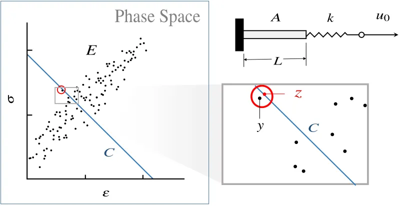
1.1 Bar loaded by soft device. The lineC is the constraint set consistent with the applied displacement u0. The material data set is the point setE. The distance minimizing, Data Driven solution is the red-encircled pointy and projectionz, which generate the
smallest distance in the phase space. . . 10
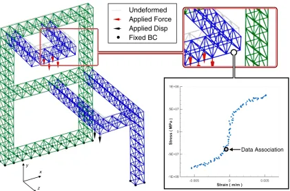
1.2 Static equilibrium of a three-dimensional truss in which the behavior of the material is known only through the data set shown. . . 11
1.3 Minimum-distance and maximum-entropy Data Driven solvers point selections for a noisy 1000 point data set . . . 13
1.4 Dynamicxdisplacement response of node at top of a base-excited truss based on noisy constitutive data. . . 15
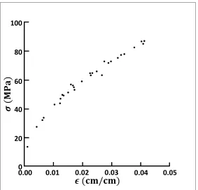
2.1 Typical material data set for truss bar. . . 19
2.2 Voronoi tessellation of a data set. . . 24
2.3 Model problem geometry with boundary conditions. . . 25
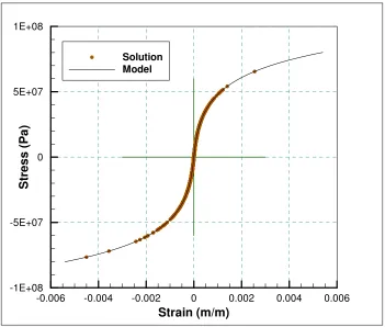
2.4 Material model with reference solution values superimposed. . . 26
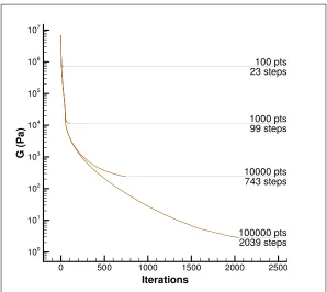
2.5 Convergence of the local data-assignment iteration. . . 27
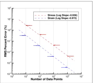
2.6 Convergence of strain and stress root-mean-square errors with number of sampling points. Histograms correspond to 30 different initial random assignments of data points to the truss members. . . 28
2.7 Typical data set with Gaussian random noise. . . 29
2.10 a) Sketch of the simulation set-up of a thin tensile specimen loaded in tension [36]. The thickness of the sample is 1 mm for the three dimensional model. b) Isometric view of the simulation set-up in 3D consisting of two rigid pins and the tensile specimen. 36 2.11 a) Coarse mesh with 811 element and an average element edge length h ≈1mm; b)
Fine mesh with 6428 elements and an average element edge length h= 0.5mm. . . 36 2.12 Linear-elastic tensile specimen. Convergence of the local material-data assignment
it-eration. FunctionalF decays through increasing data resolution in a three dimensional sampling of the plane stress space for both mesh resolutions. . . 37 2.13 Linear-elastic tensile specimen. Convergence with respect to sample size. RMS errors
decay linearly in data resolution for both stresses (σ) and strains (). . . 38 2.14 Schematic of a local material set E consisting of a finite number of states obtained,
e. g., from experimental testing. Also shown is a possible constraint set C and near intersections between E and C. . . 40 2.15 Schematic of convergent sequence of material-data sets. The parametertkcontrols the
spread of the material-data sets away from the limiting data set and the parameter ρk controls the density of material-data point. . . 45
3.1 Bar loaded by soft device. The data driven solution is the point in the material data set (circled in red) that is closest to the constraint set. . . 54 3.2 a) Geometry and boundary conditions of truss test case. b) Base material model with
reference solution stress-strain points superimposed. . . 68 3.3 Truss test case, , λ = 0.01. a) Evolution of β through the annealing schedule for
different data set sizes. b) Convergence of the max-ent Data Driven solution to the reference solution for the base model depicted in Fig. 3.2b. . . 69 3.4 Truss test case,λ= 0.1. a) Evolution ofβ through the annealing schedule for different
data set sizes. b) Convergence of the max-ent Data Driven solution to the reference solution for the base model depicted in Fig. 3.2b. . . 70 3.5 Truss test case. a) Error in the data driven solution relative to the reference solution
3.6 Truss test case. a) Random data sets generated according to capped normal distri-bution centered on the material curve of Fig. 3.2b with standard deviation in inverse proportion to the square root of the data set size. b) Convergence with respect to data set size of error histograms generated from 100 material set samples. . . 72 3.7 Truss test case. a) Random data sets generated according to normal distribution
cen-tered on the material curve of Fig. 3.2b with constant standard deviation independent of the data set size. b) Convergence with respect to data set size of error histograms generated from 100 material set samples. . . 74
4.1 a) Geometry and boundary conditions of truss test case. b) Base material model with model sampling ranges superimposed. . . 90 4.2 Truss test case. a) Random data sets generated according to capped normal
distribu-tion centered on the material curve of Figure 4.1b with standard deviadistribu-tion in inverse proportion to the square root of the data set size. b) Convergence with respect to data set size of error histograms generated from 30 material set samples. . . 95 4.3 Truss test case. a) Random data sets generated according to normal distribution
centered on the material curve of Figure 4.1b with constant standard deviation inde-pendent of the data set size. b) Convergence with respect to data set size of error histograms generated from 30 material set samples. . . 96 4.4 Data set shaded by selection frequency for a) the distance minimizing and b) entropy
maximizing selection schemes. . . 98 4.5 Max-ent displacement solutions for geometry and boundary conditions seen in
Fig-ure 4.1a solved using the data set shown in FigFig-ure 4.4 for a) the x-direction displace-ment and b) the y-displacedisplace-ment. . . 99
Chapter 1
Introduction
Significant text from this chapter is taken from [58].
1.1
Motivation
The computational sciences, as applied to physics and engineering problems, have always been con-cerned with using data inputs to provide solution results. Most of the methodologies that have been developed since the dawn of modern numerical analysis in the 1950’s have been preoccupied with the discretization of space and time. Finite differences, finite elements, finite volumes, molecular dynamics, and mesh free methods are all examples of different ways of estimating solution fields. The constitutive data that gives rise to the predictive validity of these methods has been used to create models which are then embedded into the various solution methods. These models are designed to act as succinct summaries for, at times, complicated material responses for which sum-marization is a difficult task. Machine learning has been applied to automate this sumsum-marization process, but there remain real difficulties in using reduced forms to accurately reproduce complex phenomena. Primary among issues that restrict model quality is the need to characterize responses across regimes that are data sparse. Frequently, experimental data is restricted in its ability to collect the measurements needed to fully describe the domain of interest. In cases such as this, modeling is required to both summarize data and make use of inference to operate in under-sampled regimes.
exercised to systematically generate descriptive data sets of macroscopic field response. The prob-lems for which experimental data is similarly descriptive remains comparably limited, however fu-ture experimental methods might eventually extend the range of experimentally data-characterized problems for mechanics. However, regardless of the data source, once a data set is such that data-inference is no longer required, empirical summaries are necessarily less rich than the data upon which they were based. In these circumstances, modeling then finds itself unable to take full ad-vantage of the increasingly large data sets. Ultimately, the assumed properties of a model become a restriction on the ability of a calculation to converge to measured behavior. This lack of convergence then leads to unresolvable modeling errors, which ultimately influence the quality of the calculated solution fields. The question then becomes how to move scientific computing beyond the modeling paradigm and have it operate directly on the supplied data sets. In its most general form, Data Scienceis the extraction ofknowledgefrom large volumes of unstructured data [8, 9, 7, 15]. It uses analytics, data management, statistics, and machine learning to derive mathematical models for subsequent use in decision making. Data Science already provides classification methods capable of processing source data directly into query answers in non-STEM problems, but no analogous method exists to perform scientific calculations. What remains then is a need for a method to use constitutive data to link the kinematic and kinetic laws properties which are at the core of any scientific calculation.
1.2
Thesis scope and overview
What follows in the remainder of Chapter 1 first provides descriptions of the previous Data Science applications in Section 1.3 to provide contrast to the current work. Section 1.4 then transitions to the important commonalities of Data Driven Computing methods before Section 1.5 finishes with summarized descriptions of the new methods developed in Chapters 2-4. A distance-minimizing scheme is developed in Chapter 2, which is shown to converge for sequences of data sets which uniformly converge to a functional form. Quasistatic simulations then act as the primary demonstration case for Data Driven distance-minimization. These demonstrations are replicated and extended in Chapter 3 using a max-ent based clustering argument to thermalize the method within the context of an annealing schedule. This analytic extension of the distance-minimizing solvers developed in Chapter 2 makes this new class of data solvers robust in the presence of data sequences with persistent noise. Beyond the improvement of quasistatic response for noisy data sets, this thermalized extension proves especially valuable in the multi-step evolution of dynamics calculations explored in Chapter 4.
These beginning stages of development for Data Driven Computing demonstrate new possi-bilities for a young paradigm of computational science. Chapter 5 details some of the method extensions and applications that would naturally follow from this work, as well provide concluding remarks on the work completed. Within mechanics these new methods offer the potential to provide powerful scale-linking capacity to multi-scale analysis. Data Driven solvers move constitutive data away from being a loose substrate upon which analysis resides, into becoming a core constituent of the analytical process. This process provides the techniques with new forms of causality and convergence that will make their use foundational to any number of new strategies and foci in computational prediction.
1.3
State-of-the-art and differences with previous work
1.3.1 Material Informatics
There has been extensive previous work focusing on the application of Data Science and Analytics to material data sets. The field of Material Informatics [22, 23, 69, 81, 82, 80, 84, 83, 85, 26, 73, 31, 21, 51, 50, 42, 47, 49] uses data searching and sorting techniques to survey large material data sets. It also uses machine-learning regression [19, 93] and other techniques to identify patterns and correlations in the data for purposes of combinatorial materials design and selection. These approaches represent an application of standard sorting and statistical methods to material data sets. While efficient at looking up and sifting through large data sets, it is questionable that any real epistemic knowledge is generated by these methods. What is missing in Material Informatics is a direct use – and solution of – the field equations of physics as a means of constraining and ascertaining material behaviour. By way of contrast, such field equations play a prominent role in Data Driven Computing and make the approach predictive, and not justpostdictive.
1.3.2 Material identification
There has also been extensive previous work concerned with the use of empirical data for parameter identification in prespecified material models, or for automating the calibration of the models. For instance, the Error-in-Constitutive-Equations (ECE) method is an inverse method for the identification of material parameters such as the Youngs modulus of an elastic material [41, 16, 35, 17, 20, 72, 27, 96, 10, 77, 68, 75]. While such approaches are efficient and reliable for their intended application, namely, the identification of material parameters, they are radically different from Data Driven Computing: material identification schemes aim to determine the parameters of a prespecified material law from experimental data; Data Driven Computing dispenses with material models altogether and uses material data directly in the formulation of initial-boundary-value problems and attendant calculations thereof. In particular, in Data Driven Computing no a prioriassumptions are made regarding material behaviour, and the material data that is generated and used is fundamental, unbiased, and model-independent.
1.3.3 Data repositories
mental agencies and other sources. However, it is important to note that the existing material data repositories archive parametric data that is specific to the prespecified material models, which considerably limits their value and usefulness and puts them at variance with Data Driven Com-puting. For instance, OpenKIM [1] provides parametrizations of standard interatomic potentials, such as the embedded-atom method (EAM), for a wide range of materials systems. Evidently, such data is strongly biased by the assumption of a specific form of the interatomic potential. By way of sharp contrast, Data Driven Computing supports the development of data repositories that store fundamental, unbiased, model-independent material data only. Thus, suppose that the field equations of interest are the equations of molecular dynamics. In this case, the fundamental fields are the particle position and force fields, and the local states consist of atomic positions and corresponding forces over local clusters of atoms. It thus follows that, in this case, model-free unbiased data takes the form of local atomic positions and forces, determined, e.g., by means of first-principles quantum-mechanical calculations. For more complex mesoscopic systems, the role of mathematical analysis in determining what constitutes fundamental and unbiased material data – and what unit-cell problem determines the data – is of the essence.
1.4
Problem overview of Data Driven Computating
In this secton we discuss the primary aims and requirements of solution methods as they relate to the developement of solvers which are Data Driven. While there is significant variation in how Data Driven Computing can be affected with regards to solver methodologies and application constraints, there remain commonalites whose discussion would provide clarity in the following chapters. Subsection 1.4.1 provides a description of the general nature of constituive relations in scientific computing and articulates the problems created by using models to define these relations. This is followed by Subsection 1.4.2, which discuses how Data Driven solvers relax constitutive con-straints between fields to accomodate the imposition of discrete points sets as constitutive relations. Finally Section 1.4.3 discusses the need for convergence demonstrations and their importance in underestanding the qualities of a given data solver.
1.4.1 Review of constitutive relations
1.4.2 Develping relaxation schemes
To move beyond modeling, this thesis focuses upon the material data sets upon which such a models are based. We begin by first defining a finite point set, E, which exists in phase space Z, where z= (ε, σ), and an example from small deformation mechanics would express the set as
E= ((εi, σi), i= 1,· · · , N).
The discrete nature of the set would naturally confound constitutive strategies which rely upon making use of a characterized function form. If compatibility, equilibrium, and boundary conditions are represented by the constraint set C, a problem arises in the likely case where the combined constraints cannot be satisfied by couplings defined by the discrete data set, thusE∩C returns an empty set. Knowing this, we then seek a relaxation which continues to satisfy all the members of C, while minimizing deviations from E through direct data associations.
In exploring the need for a constitutive relaxation, it is helpful to first recall how constitutive relationships are affected in spacial discretization schemes. For any fixed domain, the corresponding fields are discretely sampled for enforcement at the integration points X . Any particular spacial discretization scheme then naturally defines these points as is deemed optimal by the associated method. This sampling, later written as z∈C, is more fully expressed as
z(xi) = (ε(xi), σ(xi)),
where
X= (xi, i= 1,· · · , m),
as a means of supplying different forms of data fidelity.
1.4.3 Demonstration requirements: Data Convergence
1.5
Chapter overviews
What follows in this section is a summary of the major work topics of this thesis. To provide a greater consistency of discussion in these summaries, some of the specific examples shown here are modified versions of those seen in subsequent chapters. By providing adjacent chapter summaries here in Chapter 1, focus can be directed into distilling the top level concepts and relations that drive and connect the work in the remainder of the thesis.
1.5.1 Distance minimizing solutions
In order to add specifics to the relaxations discussed in Section 1.4.2, the question becomeshowto relatez∈C and y∈E to best reflectE as a constitutive description. The simplest demonstration of Data Driven Computing, which is discussed in Chapter 2, identifies its measure of deviation as the distance between z and y in a defined metric space, d(z, y). Thus is defined the equivalent minimization problems
min
z∈C miny∈E d(z, y) = miny∈E minz∈C d(z, y).
This formulation then defines an optimal solution which would provide the field valuesz satisfying constraintsC, and the data associationsy in the material set E.
The Data Driven Computing scheme just outlined is illustrated in Figure 1.1 by means of the elementary example of a uniformly-deformed bar deforming under the action of a loading device of known behavior. As discussed, the constraint set C and the material data setE have an empty intersection. Through the selection of a relaxed minimization criteria, an ideal solution can be identified without the crutch of an assumed constitutive form. Beyond the need for solution results to be processed directly from a material data set, a Data Driven method needs to also be capable of exhibiting data-convergence. Such convergence is shown for a sequence of data sets Ei with
corresponding size ni, where ni−1 > ni if the solution converges as i → ∞. For example, the
constraint set and data set shown in Figure 1.1 make it apparent that under a distance minimizing scheme, data-convergence would be achieved if the data sets converge to a graph in phase space.
Figure 1.1: Bar loaded by soft device. The lineC is the constraint set consistent with the applied displacement u0. The material data set is the point set E. The distance minimizing, Data Driven solution is the red-encircled pointy and projection z, which generate the smallest distance in the phase space.
truss with 1,048 degrees of freedom and a mix of specified boundary conditions. Figure 1.2 shows the geometry and boundary conditions of this test case, along with magnified deformation effects generated from the material data shown on the right. The diagram illustrates both how the con-stitutive relation of the bar is defined by a data set, and the specific nature of a data association. The distance function that defines the metric space for a stress-strain (σ,ε) phase space can be expressed as
d2(z1, z2) = E
2(ε2−ε1) 2+ 1
2E(σ2−σ1) 2,
where z = (ε, σ) and E is a selected weighting modulus. The full optimization problem then becomes
min
zdat∈Emin
n
X
e=1 we
E
2(Beu−ε
dat e )2+
1
2E(σe−σ
dat e )2
−µT
n
X
e=1
weBeTσe−f
!!
,
Figure 1.2: Static equilibrium of a three-dimensional truss in which the behavior of the material is known only through the data set shown.
the constraint set. Since the expression of all possible data associations includes all permutations of the bar-wise data assignments, the method cannot rigorously explore the entire material data space. Instead a fixed point iteration scheme is formulated to create a series of reductions in the minimizing function. This scheme, starting with an arbitrary assignment, projects the association set onto the constraint set. The projected solution is then used to perform a nearest neighbor search for new data associations. Termination then occors when all the data selections represent the closest point to their own projection.
problems.
1.5.2 Extensions to data sets with persistent noise
The initial work on Data Driven computing discussed in Chapter 2 focuses primarily on establish-ing and demonstratestablish-ing a new class of Data Driven solvers. The distance-minimizestablish-ing data solver discussed previously stands as an excellent vehicle for the exposition of this new class of methods, due in large part to the elegant simplicity of the distance-minimizing form. However, such solvers exhibit data-convergence for noisy sets only if the sequence of data sets converges to a graph in the phase space. The problem is adequately described by imagining what would happen to the data scenario pictured in Figure 1.1 if the data, instead of collapsing to a line, sees additions to the visualized set which are consistent with the pictured scatter. The points which best satisfy the constraint C would “hop” to a new point whenever one of the newly added points more closely approximates the constraint. Leaving aside the possibility of some distance ideal solution, E∩C, this process would continue indefinitely, thus preventing the convergence to a final solution. In Chapter 3, data sets which contain a finite band are accommodated using a probabilistic solution strategy which arbitrates on the relevance and importance of different data points based on prox-imity. Distance-minimizing Data Driven solvers are incapable of data-convergence for banded data sets because they seek a single data member ofE which most closely approximates the constraint set C. Cluster analysis provides a means of incorporating the influence of data neighborhoods to allow data-convergence in the presence of deeper samplings of fixed distributions.
Data Driven solvers for noisy data, developed in Chapter 3, employ cluster analysis so as to make a new kind of data driven solvers robust to outliers and is well suited to data sources with finite data bands. The foundations of cluster analysis have their roots in concepts provided by Information Theory, such as maximum-entropy estimation [52]. Specifically, we wish to quantify how well a pointzin phase space is represented by a pointziin a material data setE = (z1,· · · , zn).
Equivalently, we wish to quantify therelevanceof a pointziin the material data set to a given point
zin phase space. We measure the relevance of pointszi in the material data set by means ofweights
pi ∈[0,1] with the property: Pni=1pi = 1. We wish the ranking by relevance of the material data
to accord points distant fromzless weight than nearby points. These competing objectives can be combined by introducing a Pareto weightβ ≥0. The optimal and least-biased distribution is given by the Boltzmann distribution[89, 13]:
pi =
1
Zexp −βd 2(z, z
i)
, Z =
n
X
i=1
exp −d2(z, zi)
,
where the corresponding max-ent Data Driven solver now consists of minimizing the free energy F(z) =−logZ/βover the constraint set C. Making use of fixed point iteration, the method uses a field solutionzto weight the summed data associations, which are then projected ontoCto generate an update forz. We note that, since both methods make use of the same projection, the distance-minimizing Data Driven scheme is recovered in the limit of β → ∞. For finite β, all points in the material data set influence the solution, but their corresponding weights diminish with distance to the trial solution z. The clustering scheme just described is in analogy to information-theoretical methods for reconstructing geometrical objects and functions from point data sets [13, 32].
Strain ( m/m )
S tr e s s ( P a )
-0.04 -0.02 0 0.02 0.04
-4E+09 -2E+09 0 2E+09 4E+09 Data Min. Dist.
(a) Truss data selections using distance minimizing method
Strain ( m/m )
S tr e s s ( P a )
-0.04 -0.02 0 0.02 0.04
-4E+09 -2E+09 0 2E+09 4E+09 Data Max. Ent.
[image:25.612.77.537.372.584.2](b) Truss data selections using entropy maximizing method
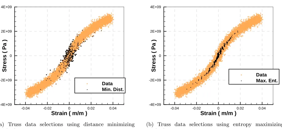
Figure 1.3: Minimum-distance and maximum-entropy Data Driven solvers point selections for a noisy 1000 point data set
provide a convex free energy after which the method proceeds to raiseβvia a sequence of contracting local convexity estimates. A free parameterλis introduced to control the speed of annealing, where solutions for a fixed data set converge under reductions to the annealing rate at significant increases to computational cost. Figure 1.3a shows the data selections made by the distance-minimizing method to solve the truss shown in Figure 1.2 from the pictured data set. In comparison, Figure 1.3b presents how the process of annealed data clustering produces selections along the center of the distribution for the same data set. Demonstrations of maximum entropy methods on the pictured static truss showed the method to data-converge faster than the equivalent distance-minimizing solver for banded data converging to a graph. Additionally, Chapter 1.3b shows the entropy maximizing method is also numerically shown to data-converge for material data sets sampled from a fixed, finitely banded, probability distribution in the phase space. While the demonstrations are computationally expensive, little effort is invested in computational efficiency and there exist several simple strategies that would greatly improve the algorithm performance. Chapter 3 ultimately presents a significant extension of Data Driven Computing to a much broader class of possible data problems.
1.5.3 Dynamics
Time (s)
D
is
p
(m
)
0 0.1 0.2 0.3 0.4
-0.1 0 0.1
[image:27.612.171.442.68.319.2]NR Soln. Max. Ent.
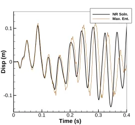
Figure 1.4: Dynamicx displacement response of node at top of a base-excited truss based on noisy constitutive data.
1.3, the deflection ux at one of the former force application points is recorded. Figure 1.4 plots
Chapter 2
Distance Minimizing Data Driven
Computing
An earlier version of this work is available as a preprint [54] and has since been published [55]. It is presented here with only small modifications.
2.1
Introduction
boundary-value problem solution methodologies, but typically with the aim of augmenting or au-tomating, rather than replacing, the use and generation of material models. Material informatics uses database techniques to first identify parameters of correlation and then use machine-learning regression techniques [19] to ultimately provide predictive quantitative models [6]. Principal-component analysis provides methods of dimensional reduction that allow such modeling techniques to be applied [31]. These approaches have been extended to the generation of multi-scale modeling correlations between macroscopic and microscopic constitutive properties [21, 46, 65, 48, 10].
These efforts may be understood as instances of Data Science, the extraction of “knowledge” from large volumes of unstructured data [9, 15]. Data science often requires sorting through big-data sets and extracting “insights” from these big-data. Data science uses big-data management, statistics and machine learning to derive mathematical models for subsequent use in decision making. Data Science currently influences primarily fields such as marketing, advertising, finance, social sciences, security, policy, medical informatics, whereas the full potential of Data Science as it relates to high-performance scientific computing is yet to be realized. Despite these limitations, reference to Data Science does effectively serve the purpose of bringing data and artificial intelligence considerations to the forefront.
data-driven problem thus consists of the minimization of a distance function to the data set in phase space subject to the satisfaction of essential constraints and conservation laws.
We provide an efficient implementation of data-driven computing and demonstrate the practi-cality of the approach is demonstrated by means of two examples of application, namely, the static equilibrium of a nonlinear three-dimensional truss and linear elasticity. In these tests, the data-driven solvers exhibit good convergence properties both with respect to the number of data points and with regard to local data assignment. The variational structure of the data-driven problem also renders it amenable to analysis. We show that, as the data set approximates increasingly closely a classical material law in phase space, the data-driven solutions converge to the classical solution. We also illustrate the robustness of data-driven solvers with respect to spatial discretiza-tion. In particular, we show that the data-driven solutions of finite-element discretizations of linear elasticity converge jointly with respect to mesh size and approximation by the data set. The math-ematical analysis is also suggestive of a number of generalizations and extensions of the data-driven computing paradigm.
2.2
Truss structures
We proceed to introduce and motivate the general approach with the aid of a simple stress-strain data set to solve a non-linear elastic truss problem. Trusses are assemblies of articulated bars that deform in uniaxial tension. Therefore, the material behavior of a bar is characterized by a particularly simple relation between uniaxial strainεand uniaxial stressσ. We refer to the space of pairs (ε, σ) as phase space. We assume that the behavior of the material of each bare= 1, . . . , m, where m is the number of bars in the truss, is characterized by—possibly different—sets Ee of
(
/
)
(
)
0.00 0.01 0.02 0.03 0.04 0.05
0 20 40 60 80 100
/
/
00.2 0.4 0.6 0.8 1.0
[image:31.612.166.449.70.342.2]0.00 0.2 0.4 0.6 0.8 1.0
Figure 2.1: Typical material data set for truss bar.
2.2.1 Data-driven solver
For a given material data set, the proposed data-driven solvers seek to assign to each bar e = 1, . . . , mof the truss the best possible local state (εe, σe) from the corresponding data setEe, while
simultaneously satisfying compatibility and equilibrium. We understand optimality of the local state in terms of an appropriate figure of merit that penalizes distance to the data set in phase space. For definiteness, we consider local penalty functions of the type
Fe(εe, σe) = min
(ε0 e,σe0)∈Ee
We(εe−ε0e) +W
∗
e(σe−σe0)
, (2.1)
for each bare= 1, . . . , min the truss, with
We(εe) =
1 2Ceε
2
e and We∗(σe) =
1 2
σ2e Ce
(2.2)
and with the minimum taken over all local states (ε0e, σ0e) in the local data setEe. We may regardWe
the functions We and We∗ are introduced as part of the numerical scheme and need not represent
any actual material behavior. In particular, the constant Ce is also numerical in nature and does
not represent a material property.
Given a global state consisting of the collection of the local states (εe, σe) of each one of its
bars, the combined penalty function
F =
m
X
e=1
weFe(εe, σe), (2.3)
penalizing all local departures of the local states of the bars from their corresponding data sets. Here and subsequently, we = AeLe denotes the volume of truss member e, with Ae its cross-sectional
area and Le its length. Therefore, the aim is to minimize F with respect to the global state
{(ε, σ)} subject to equilibrium and compatibility constraints. These aims lead to the constrained minimization problem
Minimize:
m
X
e=1
weFe(εe, σe), (2.4a)
subject to: εe= n
X
i=1
Beiui and m
X
e=1
weBeiσe=fi, (2.4b)
where {ui, i= 1, . . . , n} is the array of displacement degrees of freedom, {fi, i= 1, . . . , n} is the
array of applied forces and the coefficients Bei encode the connectivity and geometry of the truss.
The compatibility constraint can be enforced simply by expressing the strains in terms of dis-placements. The equilibrium constraint can be enforced by means of Lagrange multipliers, leading to the stationary problem
δ
m
X
e=1 weFe(
n
X
i=1
Beiui, σe)− N
X
i=1
Xm
e=1
weBeiσe−fi
ηi
!
Taking all possible variations, we obtain
δui⇒ m
X
e=1 weCe
Xn
j=1
Bejuj −ε∗e
Bei= 0, (2.6a)
δσe⇒
1 Ce
(σe−σe∗) = n
X
i=1
Beiηi, (2.6b)
δηi⇒ m
X
e=1
weBeiσe=fi, (2.6c)
where (ε∗e, σe∗) denote (unknown) optimal data points for each one of the bars, i. e., data points such that
Fe( n
X
i=1
Beiui, σe) =We( n
X
i=1
Beiui−ε∗e) +We∗(σe−σ∗e) (2.7)
or
We( n
X
i=1
Beiui−ε∗e) +W
∗
e(σe−σ∗e)≤We( n
X
i=1
Beiui−ε0e) +W
∗
e(σe−σe0) (2.8)
for all data points (ε0e, σ0e) in the local data set Ee. Once all optimal data points are determined,
eqs. (2.6) define a system of linear equations for the nodal displacements, the local stresses and the Lagrange multipliers. A straightforward manipulation of these equations renders them in the equivalent form n X j=1 m X e=1
weCeBejBei
!
uj = m
X
e=1
weCeε∗eBei, (2.9a) n X j=1 m X e=1
weCeBeiBej
!
ηj =fi− m
X
e=1
weBeiσe∗. (2.9b)
We recognize in these equations two standard linear-elastic truss-equilibrium problems with identi-cal stiffness matrix corresponding to the reference linear truss defined byWeandWe∗,e= 1, . . . , m.
The displacement problem (2.9a) is driven by the optimal local strains, whereas the Lagrange mul-tiplier problem (2.9b) is driven by the out-of-balance forces attendant to the optimal local stresses. It remains to determine the optimal local data points, i. e., the stress and strain pairs (ε∗e, σ∗e) in the local data setsEethat result in the closest possible satisfaction of compatibility and equilibrium.
The determination of the optimal local data points can be effected iteratively. Initially, all bars in the truss are assigned random points (ε∗e(0), σ
∗(0)
displacementsu(0)i and Lagrange multipliersη(0)i are then computed by solving (2.9) and the stresses σe(0) are evaluated from (2.6b). The next local data assignment is then effected by determining, for
every member in the truss, the data points (ε∗e(1), σe∗(1)) in Ee that are optimal with respect to the
local state (ε(0)e , σe(0)), i. e., such that
We(ε(0)e −ε
∗(1)
e ) +W
∗
e(σ(0)e −σ
∗(1)
e )≤We(ε(0)e −ε
0
e) +W
∗
e(σe(0)−σ
0
e) (2.10)
for all data points (ε0e, σ0e) in the local data set Ee. This operation entails simple local searches
Algorithm 1 Data-driven solver
Require: Local data sets Ee,Be-matrices, e= 1, . . . , m. Applied loads fi,i= 1, . . . , n.
i) Set k= 0. Initial local data assignment:
for all e= 1, . . . , mdo
Choose (ε∗e(0), σ∗e(0)) randomly fromEe
end for ii) Solve: n X j=1 m X e=1
weCeBejBei
!
u(jk)=
m
X
e=1
weCeε∗e(k)Bei, (2.11a) n X j=1 m X e=1
weCeBeiBej
!
ηj(k) =fi− m
X
e=1
weBeiσe∗(k), (2.11b)
foru(ik) and ηi(k),i= 1, . . . , n. iii) Compute local states:
for all e= 1, . . . , mdo
ε(ek)=
n
X
i=1
Beiu(ik), σe(k)=σ∗e(k)+Ce n
X
i=1
Beiηi(k) (2.12)
end for
iv) Local state assignment:
for all e= 1, . . . , mdo
Choose (ε∗e(k+1), σ
∗(k+1)
e ) closest to (ε(ek), σe(k)) in Ee.
end for
v) Test for convergence:
if (ε∗e(k+1), σe∗(k+1)) = (εe∗(k), σ∗e(k)) for all e= 1, . . . , m,then
v.a)ui =u(ik),i= 1, . . . , n.
v.b) (εe, σe) = (εe(k), σ(ek)),e= 1, . . . , m.
v.c)exit.
else
k←k+ 1,goto(ii).
(
/
)
(
)
0.00 0.01 0.02 0.03 0.04 0.05
0 20 40 60 80 100
/
/
00.2 0.4 0.6 0.8 1.0
[image:36.612.156.460.69.369.2]0.00 0.2 0.4 0.6 0.8 1.0
Figure 2.2: Voronoi tessellation of a data set.
The geometry of the local data assignment (2.10) is illustrated in Fig. 2.2. Thus, given a trial local state (ε(ek), σe(k)) of bare, corresponding to thekth iteration of the solver, the next data point
(ε∗e(k+1), σ∗e(k+1)) assigned to the bar is the point in Ee that is closest to (ε(ek), σe(k)) in the norm
k(εe, σe)ke=
We(εe) +We∗(σe)
1/2
. (2.13)
This is precisely the data point (ε∗e(k+1), σe∗(k+1)) in Ee whose Voronoi cell contains (ε
(k)
e , σe(k)).
Thus, the penalty function (2.1) or, equivalently, the norm (2.13) divides the phase space into cells according to the Voronoi tessellation ofEe. Each cell in that tessellation may be regarded as
2.2.2 Numerical analysis of convergence
A central question to be ascertained concerns the convergence of data-driven solvers with respect to the data set. Specifically, suppose that the materials in the truss obey a well-defined constitutive law in the form of a graph, or stress-strain curve, in (ε, σ)-phase space. Then, we expect the data-driven solutions to converge to the classical solution when the data sets approximate the stress-strain curve increasingly closely, in some appropriate sense to be made precise subsequently.
Applied Force
[image:37.612.136.477.215.599.2]Applied Displacement Fixed BC
Strain (m/m)
St
re
s
s
(P
a
)
-0.006 -0.004 -0.002 0 0.002 0.004 0.006
-1E+08 -5E+07 0 5E+07 1E+08
[image:38.612.131.482.71.369.2]Solution Model
Figure 2.4: Material model with reference solution values superimposed.
In this section, we exhibit this convergence property in a specific example of application. Fig. 2.3 shows the geometry, boundary conditions and applied loads on a truss containing 1,048 degrees of freedom. The truss undergoes small deformations and the material in all bars obeys the nonlinear non-linear elastic law shown in Fig. 2.4. A Newton-Raphson solver is used to calculate the reference solution. The reference solution values thus obtained are plotted on the constitutive stress-strain curve to show the significant amount of non-linearity seen in the solution.
Suppose that, in actual practice, the stress-strain curve in Fig. 2.4 is not known exactly but instead sampled by means of a finite collection of points, or data sets. We begin by considering a sequence (Ek) of increasingly fine data sets consisting of points on the stress-strain curve at uniform
100 pts 23 steps
100000 pts 2039 steps 10000 pts 743 steps 1000 pts 99 steps
Iterations
G
(P
a
)
0 500 1000 1500 2000 2500
100 101 102
103 104 105
106
[image:39.612.157.455.72.338.2]107
Figure 2.5: Convergence of the local data-assignment iteration.
Number of Data Points R M S P e rc e n t E rr o r (% )
102 103 104 105 106 107 10-4 10-3 10-2 10-1 100 101 102
Stress (Log Slope:-0.936) Strain (Log Slope:-0.972)
Figure 2.6: Convergence of strain and stress root-mean-square errors with number of sampling points. Histograms correspond to 30 different initial random assignments of data points to the truss members.
Next, we turn to the question of convergence with respect to the number of data points. For definiteness, we monitor the convergence of the resulting sequence of data-driven solutions to the reference solution in the sense of the normalized percent root-mean-square stress and strain errors
ε(%RMS) = 1 εref max
Pm
e=1we(εe−εrefe )2
m
1/2
, (2.14a)
σ(%RMS) = 1 σref
max
Pm
e=1we(σe−σeref)2
m
1/2
, (2.14b)
[image:40.612.158.456.72.339.2]respectively, where the maximum (εrefe , σrefe ),e= 1, . . . , mare the strains and stresses corresponding to the reference solution and (εrefmax, σrefmax) are the corresponding maximum values.
assigning data points to the truss members. Evidently, the subsequent iteration depends on this initial choice. In order to demonstrate insensitivity to such initialization, convergence plots for 30 initial random assignments are shown in Fig. 2.6 and the resulting errors are binned into histograms. The tightness of these histograms verifies the robustness of the iteration with respect to the initial data point selection.
Strain (m/m)
S
tr
e
s
s
(P
a
)
-0.006 -0.004 -0.002 0 0.002 0.004 0.006
-1E+08 -5E+07 0 5E+07 1E+08
[image:41.612.134.479.180.469.2]10000 1000 100
Figure 2.7: Typical data set with Gaussian random noise.
Next, we revisit the question of convergence with respect to the number of data points when the data set is noisy, i. e., when it does not sample the limit stress-strain curve but is offset from the curve with some probability. In this case, the data sets converge to the exact stress-strain curve as sets, in a manner to be made precise subsequently. In calculations we specifically begin by sampling the limit stress-stain curve at uniform distancesρk↓0, as in the preceding test cases, but
then add Gaussian noise to the data points of variance ρk. A typical data set is shown in Fig. 2.7
Number of Data Points
R
M
S
P
e
rc
e
n
t
E
rr
o
r
(%
)
102 103 104 105 106 107
10-4 10-3 10-2 10-1 100 101 102
[image:42.612.134.479.71.382.2]Stress (Log Slope:-0.558) Strain (Log Slope:-0.644)
Figure 2.8: Convergence of strain and stress root-mean-square errors with number of sampling points and data sets with Gaussian noise. Histograms correspond to 100 data sets.
Finally, we examine the question of sample quality, i. e., the ability of a given data set to sample closely all the local states covered by the solution. Fig. 2.9 shows the distribution of the values of the local penalty function Fe, eq. (2.1) corresponding to data sets of sizes 102, 103, 104, 105.
We recall that the value of the function Fe provides a measure of the distance of the local state
(εe, σe) to the data set. As may be seen from the figure, Fe tends to decrease with the number
of sampling points, as expected. However, for every data-set size there remains a certain spread in the values of Fe, indicating that the states of certain truss members are better sampled by the
data set than others. Specifically, truss members for which no data point lies close to their states result in high values of Fe, indicative of poor coverage by the data set. This analysis of the local
values Fe of the penalty function suggests a criterion for improving data sets adaptively so as to
ofFe. In particular, outliers, or truss members with states lying far from the data set, are targeted
for further testing. In this manner, the data set is adaptively expanded so as to provide the best possible coverage of the distribution of local states corresponding to a particular application.
weFe
10-11 10-9 10-7 10-5 10-3 10-1 101
[image:43.612.131.484.140.451.2]100000 pts 10000 pts 1000 pts 100 pts
Figure 2.9: Distribution of values of local penalty functions Fe(ε, σ) for converged data-driven
solution.
2.3
Linear elasticity
finite-dimensional by recourse to spatial discretization, the question of convergence with respect to mesh size must necessarily be elucidated within an appropriate functional framework. In this section, we extend the truss data-driven solver to linear elasticity and address the issue of data sampling in high dimensions by exploiting material and geometrical symmetry in the problem. Finally, we address the question of convergence of the finite-element discretized data-driven solver with respect to mesh size.
2.3.1 Data-driven solver
We consider a finite-element model of a non-linear elastic solid in the linearized kinematics ap-proximation. The material behavior of a solid is characterized by a relation between the strain tensor and the stress tensor σ. We refer to the space of pairs (,σ) asphase space. We assume that the behavior of the material or integration points in the model is characterized by—possibly different—setsEe of pairs (,σ), orlocal states, wheree= 1, . . . , mlabels the material points and
m is the number of material points in the finite-element model. We consider local penalty functions of the type
Fe(e,σe) = min
(0 e,σ0e)∈Ee
We(e−0e) +We∗(σe−σ0e)
, (2.15)
for each integration point e= 1, . . . , m in the solid, with
We(e) =
1
2λ(tre) 2+µ
e·e≡Cee·e, (2.16a)
We∗(σe) =
1
4µσe·σe− 1 4µ
λ
3λ+ 2µ(trσe) 2 ≡
C−e1σe·σe, (2.16b)
with the minimum taken over all local states (0e,σ0e) in the local data set Ee. We may regard We
and We∗ are reference strain and complementary energy densities, respectively.
Given a global state consisting of a collection of local states (e,σe) at each material point, we
define a global penalty function as
F =
m
X
e=1
states from their corresponding data sets. The data-driven problem is to minimizeF with respect to the global state{(,σ)} subject to equilibrium and compatibility constraints, namely,
Minimize:
m
X
e=1
weFe(e,σe), (2.18a)
subject to: e= n
X
a=1
Beaua and m
X
e=1
weBTeaσe=fa, (2.18b)
where {ua, a = 1, . . . , n} is the array of nodal displacements, {fa, a = 1, . . . , n} is the array of
applied nodal forces,nis the number of nodes and the coefficientsBeaencode the connectivity and
geometry of the solid.
As in the data-driven truss problem, the compatibility constraint can be enforced simply by expressing the strains in terms of displacements. The equilibrium constraint can in turn be enforced by means of Lagrange multipliers, resulting in the stationary problem
δ
m
X
e=1 weFe(
n
X
a=1
Beaua,σe)− N
X
a=1
Xm
e=1
weBTeaσe−fa
ηa
!
= 0. (2.19)
Taking all possible variations, we obtain the system of Euler-Lagrange equations
δua⇒ m
X
e=1
weBTeaCe
Xn
b=1
Bebub−∗e
= 0, (2.20a)
δσe⇒C−e1(σe−σ∗e) = n
X
a=1
Beaηa, (2.20b)
δηa⇒
m
X
e=1
weBTeaσe=fa, (2.20c)
where (∗e,σ∗e) denote the unknown optimal data points at material point e, i. e., the data point such that
Fe( n
X
a=1
Beaua,σe) =We( n
X
a=1
Beaua−∗e) +We∗(σe−σ∗e), (2.21)
or
We( n
X
a=1
Beaua−∗e) +W
∗
e(σe−σ∗e)≤We( n
X
a=1
Beaua−0e) +W
∗
e(σe−σ0e), (2.22)
eqs. (2.20) define a system of linear equations for the nodal displacements, the local stresses and the Lagrange multipliers. As in the data-driven truss problem, these equations can be rendered in the equivalent form
n X b=1 m X e=1
weBTeaCeBeb
!
ub= m
X
e=1
weBTeaCe∗e, (2.23a) n X b=1 m X e=1
weBTeaCeBeb
!
ηb =fa−
m
X
e=1
weBTeaσ∗e. (2.23b)
Here we recognize two standard linear-elastic equilibrium problems with identical stiffness matrix corresponding to the reference linear solid defined byWe and We∗,e= 1, . . . , m. The displacement
problem (2.23a) is driven by the optimal local strains, whereas the Lagrange multiplier problem (2.23b) is driven by the out-of-balance forces attendant to the optimal local stresses.
2.3.2 Using material symmetries to reduce data sets
Phase-space sampling requirements can be reduced if a priori knowledge of material behavior is available. In particular, material symmetry can be effectively exploited for purposes of reducing ma-terial sampling requirements. A simple and commonly encountered example of mama-terial symmetry is isotropy. For a three-dimensional isotropic material in the linearized kinematics approximation, if (e,σe) is a material data point, then so are (ReTeRe,ReTσeRe) for all rotation matrices
Re ∈SO(3), the group of proper orthogonal matrices in three dimensions. Thus, if a point (e,σe)
is in the local data setEe, then so the entireorbitof the point by SO(3).
Under these conditions, local optimality demands
Fe(e,σe) = min
(0 e,σ0e)∈Ee
min Re∈SO(3)
We(e−ReT0eRe) +We∗(σe−ReTσ0eRe)
, (2.24)
The corresponding optimality condition is ∂We
∂ij
∂ ∂Rmn
(0klRkiRlj) +
∂We∗ ∂σij
∂ ∂Rmn
(σkl0 RkiRlj)−
∂ ∂Rmn
(ΛijRkiRkj) = 0,
tives, we obtain, in matrix form,
ReT0eRe
∂We
∂e
+ReTσ0eRe
∂We∗ ∂σe
=Λ. (2.26)
Transposing both sides and using tensor symmetry we obtain
∂We
∂e
ReT0eRe+
∂We∗ ∂σe
ReTσ0eRe=Λ, (2.27)
whence it follows that
(ReT0eRe)
∂We
∂e
+ (ReTσ0eRe)
∂We∗ ∂σe = ∂We ∂e
(ReT0eRe) +
∂We∗ ∂σe
(ReTσ0eRe).
(2.28)
These equations are now to be solved for the local optimal principal directions{Re, e= 1, . . . , m},
e. g., by recourse to a Newton-Raphson iteration based on a convenient parametrization of SO(3). A simple situation arises when the local state (e,σe}is itself isotropic, i. e.,eandσe}have the
same principal directions, andWe and We∗ are chosen to be isotropic. In this case, the optimality
condition (2.28) is satisfied ifReT0eReandDWeandReTσ0eReandDWe∗commute, which in turn
holds if and only ifReT0eReandeandReTσ0eReandσehave the same eigenvectors. Introducing
the representations
e=QeTeeQe, σe=QeTseQe,
0e=Q0eTe0eQ0e, σ0e=Q0eTs0eQ0e,
(2.29)
withQe,Q0e∈SO(3) andee,se,e0e,s0e diagonal, local optimality then requires
Re =Q0eQe−1, (2.30)
which determines explicitly the optimal data point in theSO(3)-orbit of (e0e,s0e).
In general, since the local states (e,σe} follow from independent Euler-Lagrange equations,
2.3.3 Numerical analysis of convergence
44 60
8 R10
R2
1
5
2
2 2
(a) (b)
Figure 2.10: a) Sketch of the simulation set-up of a thin tensile specimen loaded in tension [36]. The thickness of the sample is 1 mm for the three dimensional model. b) Isometric view of the simulation set-up in 3D consisting of two rigid pins and the tensile specimen.
[image:48.612.82.538.113.280.2](a) (b)
Figure 2.11: a) Coarse mesh with 811 element and an average element edge length h ≈1mm; b) Fine mesh with 6428 elements and an average element edge lengthh= 0.5mm.
three-elements containing eight Gauss quadrature points each.
Sampling requirements are reduced by virtue of the plane-stress conditions of the problem under consideration. Specifically, only a neighborhood of the subspaceσ13=σ23=σ33= 0 in stress space needs to be covered by the data. We accomplish this requirement by sampling an appropriate region of the (σ11, σ22, τ12) stress plane on a uniform cubic grid. The corresponding strains (11, 22, 12) then obey an isotropic linear-elastic law. A reference isotropic linear-elastic solid of the type (2.16), unrelated to the actual material behavior sampled by the material data, is used in the data-driven calculations. These reductions effectively limit the material data set to a three-dimensional space.
Number of Steps
F
2 4 6 8 10 12 14 16 18
102
103
104
105
106
Course Mesh Fine Mesh
123pts
243pts
483pts
963pts
[image:49.612.133.482.240.552.2]1923pts
Figure 2.12: Linear-elastic tensile specimen. Convergence of the local material-data assignment iteration. Functional F decays through increasing data resolution in a three dimensional sampling of the plane stress space for both mesh resolutions.
iteration for both mesh resolutions on increasingly large data sets. The number of iterations to convergence increases with the material-data sample size but, remarkably, remains modest in all cases.
(Number of Data Points)1/3
R
M
S
P
e
rc
e
n
t
E
rr
o
r
(%
)
100 200 300
10-1 100 101
Course Stress (Log Slope: -0.902) Course Strain (Log Slope: -1.067) Fine Stress (Log Slope: -0.910) Fine Strain (Log Slope: -1.060)
[image:50.612.129.483.137.445.2]10 50
Figure 2.13: Linear-elastic tensile specimen. Convergence with respect to sample size. RMS errors decay linearly in data resolution for both stresses (σ) and strains ().
To calculate percent error with respect to the reference solution we re-define the RMS error metric as
σ(%RM S)=
Pm
e=1weW
∗σ
e−σrefe )
Pm
e=1weW∗(σrefe )
1/2
, (2.31a)
(%RM S)=
Pm
e=1weW(e−refe )
Pm
e=1weW(refe )
1/2
, (2.31b)
keeping with the analytical estimate of Corollary 1.
2.4
Mathematical analysis of convergence
We proceed to abstract from the preceding examples a general class of data-driven problems and to establish some of their fundamental properties by way of analysis. We consider systems whose state is characterized by points points in a certain phase spaceZ. For instance, in the case of linear elasticity, the system of interest is an elastic solid occupying a certain domain Ω and the state of the system is defined by the pair (,σ), where is the strain field and σ is the stress field, both defined over Ω. In this case, the phase spaceZ of the elastic solid is an appropriate space of pairs (,σ) of strain and stress fields over Ω.
We particularly wish to characterize the states of the system that are in a constraint set C of states satisfying essential constraints and conservation laws. For instance, in the running example of linear elasticity we may wish to determine states (,σ) ∈Z satisfying compatibility, i. e., such that
(x) =1/2 ∇u(x) +∇uT(x), x∈Ω, (2.32a)
u(x) = ¯u(x), x∈∂ΩD, (2.32b)
for some displacement fieldu over Ω and prescribed displacements ¯u over the Dirichlet boundary ∂ΩD, and satisfying equilibrium, i. e., such that
∇ ·σ(x) +f(x) =0, x∈Ω, (2.33a)
σ(x)n(x) = ¯t(x), x∈∂ΩN, (2.33b)
for some applied body force fieldf over Ω and tractions ¯tover the Neumann boundary∂ΩN, with
unit outer normal n.
Classically, the problem is closed by putting forth a material law restricting the set of admissible states to a graphE inZ. For instance, in linearized elasticity the material law may take the form a nonlinear Hooke’s law
σ(x) =DW (x)
where W is the strain-energy density of the material. The set E then consists of the set of strain and stress fields satisfying the material law at all material points in Ω. The classical solution set is then the intersection E∩C, consisting of states of the system satisfying the essential constraints, the conservation laws and the material law simultaneously. In the case of linear elasticity, the classical solutions would consist of compatible strain fields and equilibrium stress fields satisfying the material law at all material points. In general, the cardinality of the solution setE∩Cdepends on the transversality of C with respect to E, depending on which, the solution set may be empty or non-empty, in which latter case the solution set may consist of a single point, corresponding to a unique classical solution, or multiple points.
(
)
0.00 0.01 0.02 0.03 0.04 0.05
0 20 40 60 80 100
C
=
∩
E
[image:52.612.156.459.262.554.2](
/
)
Figure 2.14: Schematic of a local material set E consisting of a finite number of states obtained, e. g., from experimental testing. Also shown is a possible constraint set C and near intersections betweenE andC.
of experimental testing, cf. Fig. 2.14. Under such conditions, E∩C is likely to be empty even in cases when solutions could be reasonably expected to exist. It is, therefore, necessary to replace the overly-rigid problem of determining E∩C by a suitable penalizationthereof. To this end, we begin by introducing a norm | · |in phase space. For instance, for truss structures we may choose
|x|2 =
m
X
e=1 we
Ceε2e+
σe2 Ce
, (2.35)
withx≡(e, σe)me=1 denoting a generic point in phase spaceZ. For discretized linear-elastic solids we may choose
|x|2 =
m
X
e=1
we Cee·e+C−e1σe·σe
, (2.36)
with elabeling the integration points in the discretization and x ≡(e,σe)me=1 denoting a generic point in phase spaceZ. Finally, for continuum linear elasticity we may choose
|x|2 =
Z
Ω
C(x)(x)·(x) +C−1(x)σ(x)·σ(x) dx. (2.37)
withx≡ { (x),σ(x), x∈Ω} denoting a generic point in phase spaceZ.
Based on this metrization of phase space, we define the data-drive problem as the double minimum problem
min
y∈Eminx∈C|y−x|= miny∈Edist(y, C), (2.38)
or, equivalently,
min
x∈Cminy∈E|x−y|= minx∈Cdist(x, E). (2.39)
Thus, the aim of the data-driven problem, as expressed in (2.38), is to find the point in the material-data set that is closest to satisfying the essential constraints and conservation laws, or, as expressed in (2.39), to find the point in the constraint set that is closest to the material-data set. In the particular example of linear elasticity, the aim of the data-driven problem, as expressed in (2.38), is to find the point in the material-data set that is closest to being compatible and in equilibrium, or, as expressed in (2.39), to find the compatible equilibrium point that is closest to the material-data set.
examples of (2.38) and (2.39) with norms (2.35) and (2.36), respectively.
2.4.1 Finite-dimensional case: Convergence with respect to sample size
We begin by considering systems whose local states take values in a finite-dimensional phase space Z. The global state of the system is then characterized by a point x∈Z, where m is the number of material points of the system. The essential constraints and conservation laws pertaining to the system have the effect of constraining its global state to lie on a subsetC of Z. For instance, for linear-elastic trusses such as considered in the preceding section, the local phase spaceZe of bare
is the space of pairs (, σ)∈R2, whereis axial strain of a bar andσthe corresponding axial stress. The global phase space of the entire truss is thenZ=Z1× · · · ×Zm, wheremis the number of bars
in the truss. In addition, the constraint set C is the affine space of compatible and equilibrated states of stress and strain in the truss.
The data-driven problem (2.38) is now formulated by specifying a set E of possible material states inZ. For instance, in the case of a truss a local material setEeof the form shown in Fig. 2.14
may be supplying for every bareof the truss and the global material set is thenE =E1× · · · ×Em.
We note that, ifE is compact, i. e., consisting of a finite collection of points, then the corresponding data-driven problem has solutions by the Weierstrass extreme-value theorem.
We proceed to consider the question of convergence with respect to the data set. Specifically, we suppose that a sequence (Ek) of data sets is supplied that approximates increasingly closely
a limiting data set E. The particular case in which E is a graph concerns convergence of data-driven solutions to classical solutions. For instance, the approximations (Ek) may be the result of
an increasing number of experimental tests sampling the behavior of a material characterized by a—possibly unknown—stress-strain curveE. The sequence of approximate material data sets (Ek)
generates in turn a sequence of approximate problems
min
xk∈C
min
yk∈Ek
|xk−yk|, (2.40)
and attendant approximate solutions (xk). We wish to ascertain conditions under which (xk)
converges to solutions of the E-problem.
follow-E ⊂Z, i. e.,
dist(x, E) = inf
y∈E|x−y|, (2.41)
and by PYx the projection ofx∈Z onto a subspaceY of Z, i. e.,
|x−PYx|= dist(x, Y). (2.42)
Proposition 1. Let (Ek) be a sequence of finite subsets of Z, E a subset of Z and C a subspace
of Z. Letx be an isolated point of E∩C and letxk, yk∈Z be such that
(xk, yk)∈argmin{|x−y|, x∈C, y∈Ek}. (2.43)
Suppose that:
i) There is a sequence ρk↓0 such that
dist(z, Ek)≤ρk, ∀z∈E. (2.44)
ii) There is a sequence tk↓0 such that
dist(zk, E)≤tk, ∀zk∈Ek. (2.45)
iii) (Transversality) There is a constant 0≤λ <1 and a neighborhood U of x such that
|PCz−x| ≤λ|z−x|, (2.46)
for allz∈E∩U. Then,
|xk−x| ≤
tk+λ(tk+ρk)
1−λ , (2.47)
and, therefore, limk→∞|xk−x|= 0.
Proof. By assumption (i), we can find zk∈Ek such that
Figure


Outline
Related documents
