University of Huddersfield Repository
Anyakwo, Arthur, Pislaru, Crinela, Ball, Andrew and Gu, Fengshou
A Novel Approach To Modelling And Simulation Of The Dynamic Behaviour Of The WheelRail
Interface
Original Citation
Anyakwo, Arthur, Pislaru, Crinela, Ball, Andrew and Gu, Fengshou (2011) A Novel Approach To
Modelling And Simulation Of The Dynamic Behaviour Of The WheelRail Interface. In:
Proceedings of the 17th International Conference on Automation & Computing. Chinese
Automation and Computing Society, Huddersfield. ISBN 9781862180987
This version is available at http://eprints.hud.ac.uk/id/eprint/11492/
The University Repository is a digital collection of the research output of the
University, available on Open Access. Copyright and Moral Rights for the items
on this site are retained by the individual author and/or other copyright owners.
Users may access full items free of charge; copies of full text items generally
can be reproduced, displayed or performed and given to third parties in any
format or medium for personal research or study, educational or notforprofit
purposes without prior permission or charge, provided:
•
The authors, title and full bibliographic details is credited in any copy;
•
A hyperlink and/or URL is included for the original metadata page; and
•
The content is not changed in any way.
For more information, including our policy and submission procedure, please
contact the Repository Team at: [email protected].
A NOVEL APPROACH TO MODELLING AND SIMULATION OF THE
DYNAMIC BEHAVIOUR OF THE WHEEL-RAIL INTERFACE
Arthur Anyakwo, Crinela Pislaru, Andrew Ball, Fengshou Gu University of Huddersfield
Diagnostics Engineering Research Centre Queensgate, Huddersfield, HD1 3DH
Abstract— This paper presents a novel approach to modelling and simulation of the dynamic behaviour of rail-wheel interface. The proposed dynamic wheel-rail contact model comprises wheel-rail geometry and efficient solutions for normal and tangential contact problems. This two-degree of freedom model takes into account the lateral displacement of the wheelset and the yaw angle. Single wheel tread rail contact was considered for all simulations and Kalker‟s linear theory and heuristic non-linear creep models were employed. The second order differential equations are reduced to first order and the forward velocity of the wheelset is increased until the wheelset becomes unstable. A comprehensive study of the wheelset lateral stability is performed and is relatively easy to use since no mathematical approach is required to estimate the critical velocity of the dynamic wheel-rail contact model. This novel approach to modelling and simulation of the dynamic behaviour of rail-wheel interface will be useful in the development of intelligent infrastructure diagnostic and condition monitoring systems. The automated detection of the state of the track will allow informed decision making on asset management actions – especially in maintenance and renewals activities.
Keywords: modelling; simulation; condition monitoring; systems engineering; wheel-rail contact
NOMENCLATURE
R0 = Nominal rolling radius of the wheel (460mm) Rl = left wheel rolling radius (mm)
Rr = Right wheel rolling radius (mm) RraiL = Rail radius (79.37 mm)
a = Half length of the semi-axes of c in the rolling direction (mm)
b = Half length of the semi-axis of contact patch in the lateral direction (mm).
Iz = Moment of Inertia of the wheelset (700x106kg-mm2) Kpy = Lateral suspension stiffness (3.86x10³N/mm) Kpx = Longitudinal spring stiffness (850N/mm) Cpy = Lateral damper coefficient (8 Ns/mm) Cpx = Longitudinal damper coefficient (100 Ns/mm) f11 = Longitudinal linear creep coefficient (8.06x10⁶ N) f22 = Lateral linear creep coefficient (8.09 x 10⁶N) f23 = Lateral/spin linear creep coefficient (2.2 x 10⁷ N-mm) f33 = Spin linear creep coefficient (1.27x10
7
Nmm2)
m = Mass of the wheelset (1250kg)
W = Axle load (110,000N)
vx = longitudinal creepage vy = lateral creepage vspin = Spin creepage
l0 = Half wheel axle length in central position (742.9mm)
G = Shear Modulus of rigidity = 80x103MPA
C11 = Longitudinal creep coefficient C22 = Lateral creep coefficient C23 = Lateral/spin creep coefficient C33 = Spin linear coefficient
d = Half distance between the two springs (900mm)
l0 = Half wheelset axle distance (742.9mm)
= Roll velocity
I. INTRODUCTION
The lateral stability of the wheelset affects the dynamic motion of the railway vehicle. This phenomenon depends on the wheel-rail contact model, wheel-rail profile design, hunting, critical velocity and creep contact forces acting on the contact patch. Hertz theory was applied to solve wheel-rail contact problems [1]. Hertz model runs very fast in real time and is thus used in most railway vehicle dynamic simulations. However for rapidly changing contacts with time and with increased normal contact forces, Hertz model is not suitable since in these situations the contact region becomes conformal. Semi-Hertzian method [2-3] was developed to cater for the variations and increase in the normal contact forces acting on the wheel-rail interface. It uses the geometric intersection of two solids in contact region to find out the shape of the contact patch. Kalker, [4] proposed the exact theory of the wheel-rail contact model by developing a robust algorithm called CONTACT. This model requires so much computation power since the contact patch is discretized into stripes before the tangential creep forces are calculated. Finite Element Method (FEM) [5] was used to model the dynamics of the wheel-rail interface. Due to the enormous computational time required to implement FEM methods, it rarely used for railway vehicle dynamic simulations.
The tangential creep forces play a vital role in wheel-rail rolling theory. Carter solved the 2-Dimensional problem of wheel-rail contact rolling theory using a locomotive wheel and a cylindrical rail [6]. He maintained the fact that the tangential creep forces must not exceed the Coulombs maximum limit. Johnson and Vermeulen extended Carter‟s theory to 3-dimensional case to include the two smooth half rolling surfaces without spin. Carter‟s model considered only the relationship between the longitudinal creepage and the tangential forces on the contact patch region. Kalker [7] proposed the linear theory for determining the tangential forces acting on the contact patch. A new Heuristic non-linear model [8-9] Proceedings of the 17th International Conference on
developed by Shen for limiting the tangential forces is discussed. Several dynamic models have been developed for wheel-rail interface using the wheel-rail profile geometry. A parametric 3-dimensional wheel-rail contact model was developed to model the dynamics of the wheel-rail contact model [10]. Wickens [11] studied the effect on hunting on a railway vehicle on a straight track. He observed that hunting motion occurs when the critical velocity of the wheelset exceeds the maximum required speed limit of the designed for its operation. Finally a new model was developed to study the dynamic interaction of the wheel-rail contact on a curved track [12]. This study showed that the lateral and longitudinal stiffness has significant effect on critical velocity of the railway vehicle.
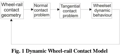
[image:3.596.75.278.394.485.2]In this paper a two dimensional wheel-rail contact model is modeled. Hertz contact model is used to get the contact patch size dimensions and then the Heuristic nonlinear model is applied to limit the creep contact forces. The lateral stability of the wheelset is investigated by solving the system of non-linear equations of the model using Runge-Kutta‟s method. The lateral stability of the wheelset is then investigated by increasing the forward velocity of the wheelset until it becomes unstable. The proposed model contains; wheel-rail contact geometry, normal and tangential contact problems and equations for describing the dynamic equation (see Fig. 1).
Fig. 1 Dynamic Wheel-rail Contact Model
II. WHEEL-RAILCONTACTGEOMETRY
A new conical wheel profile with wheel tread taper 1:20 is used to model the dynamic wheel-rail contact model. A BS 113A rail profile is also used for the model of the rail-profile. The nominal rolling radius Ro of the wheelset is 460mm while the rail radius Rrail in contact point range is 79.37mm as shown in Fig. 2. This is the contact point range for the wheelset on the track.
Assuming that the yaw angle of the wheelset is very small and can be neglected, the 2-Dmensional model of the wheel-rail contact geometry considering the vertical displacement uz and the lateral displacement uy is modeled (see Fig. 3).
The railway track is considered to be rigid and there is no cant applied at both rails. When the wheelset is in central position, the angle made by the horizontal plane is wr for the right wheel and wl for the left wheel. Similarly, the co-ordinate of point A at central position with respect to the wheelset frame is (l0, -R0). When the wheelset is displaced laterally from its central position to the right (as shown in Fig. 3) the rail contact slope formed by the new wheel rail contact point B from A for right wheel profile is rr. It is a function of the roll angle and the wheel contact slope wr. The rolling radius for the right and left wheel tread becomes Rr and Rl. The previous wheel-rail contact point on the wheel is now contact point C (see Fig. 3).
The wheel-rail co-ordinates are defined (see Fig. 2) as follows
wr = Right wheel co-ordinate (lateral direction)
rr = Right rail co-ordinate (lateral direction)
wr = Right wheel co-ordinate (vertical direction)
rr = Right rail co-ordinate (vertical direction) uz = Vertical displacement
uy = Lateral displacement
The lateral distance between point A and C is
0 l sin ) 0 R z u ( cos ) 0 l y u ( 0 l c Y c
Y
(1)
Similarly, the total vertical distance from point A to C is
0 cos ) 0 ( sin ) 0 ( ) 0
( R R
z u l
y u R c Z c
Z
(2)
Fig. 3 Right wheel rail geometry
The total lateral distance between point B and C is
0 ) rr c Δ ( sin wr cos
wr
Y (3)
Also, the vertical distance between point B and C is
0 ) rr c (Δ cos wr sin
wr
Z (4)
where Zc and Yc are the vertical and lateral co-ordinates at point C.
For small roll angles cos = 1, and sin = 0, Eq. 3 and Eqn. 4 simplifies to
0 rr wr wr
0
z
u R
y
u (5)
rr y
u l
z
u
wr wr
0 (6)
The right rail contact slope rr (see Fig. 3) is
wr
rr (7)
Similarly the equations for the left hand wheel-rail contact geometry are
0 l w l r z u l w 0 R y
[image:3.596.58.289.646.761.2]u (8)
0 l w l r l w y u l z
u
0 (9)
wl δ rl
δ (10)
Assuming that the contact points are constrained between the region of -14.13mm <
wr < 1.48mm and -1.48mm <
wl < 14.13mm for the right and left wheel profile, thenthe wheel profile equations is
0 05 . 0 wr wr
(11)
0 05 . 0 wl wl
(12)
The BS 113A rail profile is made up of three main curves with rail radius of 79.37mm, 304.8mm, 79.37 mm (see Fig. 2). The equation of the curves for the region
-14.13mm <
rr < 1.48mm, right rail contact point regionand -1.48mm <
rl < 14.13mm, left rail contact pointregion can be defined as follows;
2 / 1 ) 2 ) 96 . 3 rr ( 2 37 . 79 ( 27 .
79
rr (13)
2 / 1 ) 2 ) 96 . 3 r ( 2 37 . 79 ( 27 .
79
l
rl
(14)
The wheel contact slope is defined as
05 . 0
/
wr d wr d
wr
(15)
05 . 0 /
wl d wl d
wl
(16)
2 1 2 96 3 2
37 79 96
3 . ) ) /
rr ( .. /( ) . rr ( rr d / rr d
rr
(17)
2 1 2 96 3 2
37 79 96
3 . ) ) /
rl ( .. /( ) . rl ( rl d / rl d
rl
(18)
Equations (5) to (18) can be solved synchronously taking uy as the input variable using Newton‟s method which is discussed next.
A. Numerical Solution (Newton Raphson Method)
Several methods exist for solving non-linear multi-dimensional equations. The two most common methods include the Newton Raphson‟s method and the Quasi-Newton method. Quasi-Newton Raphson method is a numerical method for solving simultaneous non-linear equations. It provides quadratic convergence of the solutions provided the initial conditions are close to the actual solution [15]. The algorithm for implementing this method is
) k x ( f J k x k
x 1
1
(19)
where
J-1 = Inverse Jacobian matrix of f(xk)
xk = initial guess used as the starting point for iterations xk+1 = the new guess
The Newton Raphson algorithm terminates only when the function f(x) is close to zero. The value of x at that point is obtained as the solution to the equation. For application to solving the wheel-rail contact geometry equations, Newton Raphson‟s method is less efficient since for every lateral displacement input uy, the initial conditions must be guessed to ensure quick convergence to the solution. A better method for solving these equations is the Quasi-Newton method [15].
B. Quasi Newton Method
The Quasi-Newton method is an optimization technique that can be used to solve a system of non-linear differential equations. In Newton-Raphson‟s method, the Jacobian matrix had to be computed in every iteration but with the Quasi-Newton method, a single Jacobian matrix is determined and thus used for iteration. In Matlab, the function fsolve is used to solve a set of simulations non-linear equations using Quasi-Newton‟s theory of the form
f(x) = 0; (20)
The algorithms implemented in fsolve function are Gauss-Newton method, Levenberg-Marquardt method and the Trust-Region-Reflective method [14]
The syntax used for implementation in Matlab is [14]; x = fsolve (function, x0, options) (21) where
x = solution of the equation in vector form
function = function file containing the set of non-linear simultaneous equations
x0 = the initial condition of x
options = optimization options used for simulations. Writing the wheel-rail geometry equations into a function file and solving using initial conditions x0 equal to zeros all through, the wheel-rail co-ordinates converged easily to the solution.
For the dynamic wheel-rail contact model, the two most important parameters that are required are the contact angle and the rolling radius difference of the curve. The contact angle for the left and right wheel-rail geometry defined in Eqn. (7) and (10) would be used for the dynamic model simulation. The rail contact angle plot for the left/right wheel contact is shown below
Identify applicable sponsor/s here. (sponsors)
Fig. 5 Contact angle (left and right wheel-rail contact)
[image:4.596.319.530.461.579.2] [image:4.596.310.535.610.730.2]Fig. 6 shows the Rolling radius difference of the wheelset derived from the left and right vertical wheel co-ordinates wr and wlas follows
wr R r
R
0 (22)
wl R l
R
0 (23)
The flangeway clearance for this model is 13mm. Single wheel-rail contact simulations is considered in the wheel tread region for the left and right wheel.
III THE NORMAL CONTACT PROBLEM
For an applied load on a wheel-rail interface, Normal contact forces develop on the contact patch depending on the total vertical force applied and the contact angle of the wheel-rail contact formed as a result of the lateral displacement y of the wheelset during motion (see Fig. 7).
The normal contact forces acting on the left and right wheel in static equilibrium is Qr and Ql given as
l Q ) l w cos( l
N (24)
r Q ) wr cos( r
N (25)
The lateral forces Fyr and Fyl can be resolved as follows assuming small roll angles
yr F ) l w sin( l
N
(26)
yl F ) wr sin( r
N (27)
The total lateral force acting on the contact patch is
) wr tan( r Q ) wr tan( l Q yl F yr
F (28)
For small contact angles
W yl F yr F
Gr (29)
Gr is the gravitational force. The Gravitational force restores the wheelset back to its central position when it is displaced in the lateral direction.
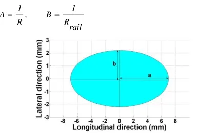
A. Hertz Contact Model
Hertz contact theory predicts the size of the contact patch using the following formulae;
3 2
2 2 1 3
/
N ) B A ( E
) u ( mn ab
(30)
where m and n are the Hertz elliptical constants [2], N is the normal force(left and right wheel-rail) acting on the contact patch and A and B are the relative curvatures given as
rail R
1 B , R 1
A (31)
R is the Nominal rolling radius at left and right wheel in the central position or the rolling radii of the left and right wheel as a result of lateral displacement. Rrailis the radius of the rail. In Fig. 8, the Elliptical contact patch for the wheel-rail contact model is shown with values a = 7.0045mm and b = 2.20245mm. Poisson‟s ratio (u = 0.3) and Young Modulus (E = 210000MPA).
IV TANGENTIAL CONTACT PROBLEM
The tangential contact problem resolves the tangential creep forces acting on the contact patch. A deviation from pure rolling motion of the wheelset is caused by acceleration, traction, braking and the presence of lateral forces acting on the wheel-rail interface. Creepages are thus formed as a result and can be represented as
creepage) al
longitudin (
v 2x v 1x v
x v
(32)
v 2y v 1y v
x v
(Lateral creepage) (33)
v 2 1 spin v
(Spin creepage) (34)
where v is velocity and v2x, v2y, 2 are the real velocities while v1x, v1y, 1 are the pure rolling velocities of the wheels in the absence of creep. The longitudinal creepages at (right and left) wheel-rail contact
v ψ 0 l ) 0 /R l R -v(1
xl v , v
ψ 0 l -) 0 /R r R -v(1
xr v
(35)
The lateral creepages at the right and left wheel-rail contact
φ 1 v ) 0 /R r ψ)(R y -1 (v yr
v (36)
φ 1 v ) 0 /R l ψ)(R y -1 (v yl
v (37)
The spin creepages at the right and left wheel-rail contact is
) 0 λ/R ψ 1 (v spinr
v (38)
) 0 λ/R ψ 1 (v spinl
[image:5.596.59.260.267.382.2]v (39)
Fig. 8 Elliptical Contact Patch for 0mm lateral displacement (Left/Right wheel-rail contact)
Fig. 7 Vertical and Normal Contact forces acting on
[image:5.596.55.289.398.619.2]A. Kalker’s Linear Theory
Kalker established a linear relationship between the developed creepages at the contact patch and the creep forces [7]. The maximum creep forces as determined by Kalker are as follows
Longitudinal creep force
xr v 11 f xr
F (40)
xl v 11 f xl
F (41)
Lateral creep force
spinr v 23 f yr v 22 f yr
F (42)
spinl v 23 f yl v 22 f yl
F (43)
Spin creep moment
spinr v 33 f yr v 23 f zr
M (44)
spinl v 33 f yl v 23 f zl
M (45)
where
33 23 22 11,f ,f ,f
f are the linear creep coefficients
given computed as
11 11 GabC
f (46)
22 22 GabC
f (47)
23 5 1 23 C . ) ab ( G
f (48)
33 2 33 G(ab) C
f (49)
33 23 22 11,C ,C ,C
C are the creep coefficients tabulated by
Kalker [6] and G is the Shear modulus of rigidity of steel.
B Heuristic Non-linear Model
The Heuristic non-linear creep model was developed by Shen and White [8] to cater for the non-linearities in the wheel-rail geometry, adhesion limits on the creep force-creepage relationship and the spin force-creepage effect. The creep forces developed by Kalker‟s linear theory are limited for high creepages by a saturation constant „a‟ developed as follows;
3 1 3 3 1 27 2 1 3 1 , ), ( a (50)where (i r,l j r,l)
N ) yj F ( ) xi F ( 2 2 (51)
= unlimited normalized creep ratio The reduced creep forces now become
x aF r x
F (52)
y aF r y
F (53)
z aM r z
M (54)
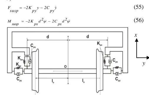
V WHEELSET DYNAMIC BEHAVIOUR
The dynamic behaviour of the wheelset is studied by summing the total forces acting on the wheelset and then applying Newton‟s law. In this paper the suspended wheelset is used which includes the primary suspensions
in the longitudinal and lateral direction. The top view of the suspended wheelset is shown below where x is the rolling direction and y is the lateral direction.
The suspension forces in the lateral direction and longitudinal direction can be resolved as follows (see Fig. 9) y py C 2 y py K 2 susp
F (55)
d2
px C 2 2 d px K 2 susp
M (56)
The equations of motion of the can be derived by combining Eqns. (40 – 45, 55-56) to arrive at the Kalker linear model. For the Heuristic nonlinear model, Eqns. (52-54) is used to replace the maximum creep forces computed in Eqns. (40 – 45). Neglecting the effect of the gyroscopic wheel moment, the two degree of freedom equations of motion comprising of the lateral displacement y, and the yaw angle are defined as follows 0 ψ 22 2f Wλλ) 1 0 l py (2K ψ 1 v 33 2f y ) py 2C λ 0 R 1 0 l (1 1 v 22 2f y m (57)
The yaw rotation equation of motion is
0 )ψ o Wλλ 2 d px 2K 22 (2f o λ/R o l 11 2f ψ ) 2 d px C * 2 )/v 11 f 2 o l 2(f11 y ) o l o λv/R y I λ 0 R 1 0 l (1 1 v 23 2f ψ z I (58)
A. Equations of Motion
The equations of motion of the suspended wheelset Eqn. (50)-(51) is can reduced to a system of first order differential equations;
x(t) f (t)x (59)
where x(t) is a 4 x 1 state vector variable.
VI SIMULATED RESULTS
The ODE45 function in MATLAB implements Runge Kutta 4th order method with variable time step for computational efficiency [14]. It solves initial value problems of the form
x) f(t, (t)
x , x(t0) = x0 (60) where x is a state vector of the dependent variables and t is the independent variable [14].
[image:6.596.296.549.140.301.2]Applying Ode45 function to solving the equations of motion, the syntax used is
Fig. 9 Top view (Suspended Wheelset diagram) x
[t,x] = ode45 (@fun, tspan, initialconditions)
Where fun = function file contain the reduced first order differential equations of motion for the system
tspan = time span for simulation (30 seconds)
initialconditions = initials conditions required for simulation of the dynamic wheel-rail contact model. The state variables used for simulation is
x(1) = Lateral displacement (Initial condition = 5mm) x(2) = Yaw angle (Initial condition = 0)
x(3) = Lateral velocity (Initial condition = 0) x(4) = Yaw velocity (Initial condition = 0)
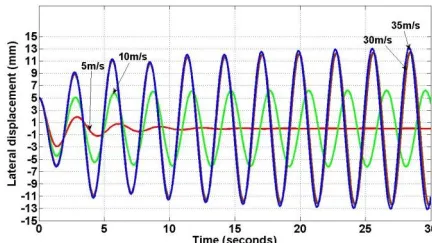
[image:7.596.74.288.434.556.2]Further details on the use of Ode45 function can be found in [14]. Fig. 10 and Fig.11 shows Kalker linear Model and the Heuristic Non-linear Model results for various forward velocity inputs. Increasing the forward velocity of the wheelset from 5m/s (5000mm/s) to 40m/s leads to increasing amplitude peaks until the critical velocity is reached. For Kalker‟s linear model, the critical velocity just before flange contact is 40m/s while for the Heuristic Non-linear model, the critical velocity just before wheel flange contact is 35m/s. It can be readily noted that the critical hunting speeds of the linear model is generally slightly higher than the critical speed for the Heuristic non-linear model. Therefore increase in the forward speed of the wheelset leads to lateral instability and hunting. In most real situations the gravitational forces act as a restoring force to limit these increasing lateral oscillations.
Fig. 10 Lateral displacement of the wheelset for initial velocity 10, 30, 40m/s (Kalker’s linear Model)
Fig. 11 Lateral displacement of the Wheelset for initial velocity 10, 30, 40m/s (Heuristic Non-linear Model)
VII CONCLUSIONS
In this paper, a new dynamic wheel-rail contact model was developed to study the lateral stability of the wheelset on the track. The equation of motion of a two degree of freedom single suspended wheelset model was derived completely. It was found that as the forward velocity of the wheelset increases, the wheelset becomes unstable on the track due to increasing lateral oscillations. These oscillations are limited by flange contact. This novel approach to modelling and simulation of the dynamic behaviour of rail-wheel interface will be useful in the development of intelligent infrastructure diagnostic and condition monitoring systems.
REFERENCES
[1] W. Yan, and F. D. Fischer, “Applicability of Hertz Contact
theory to rail-wheel contact problems,”Archive of Applied Mechanics, vol. 70, May 1999, pp. 255–268.
[2] J. B. Ayasse, and H. Chollet, “Determination of wheel-rail contact patch in semi-Hertzian Conditions”, Vehicle System Dynamics, vol. 2. Oxford: Number 2, March 2005, pp. 161 – 172.
[3] X Quost, M. S, A. Eddhahak, J.B. Ayasse, H. Chollet, and P.E. Gautier, “Assessment of the semi-Hertzian method for the determination of the wheel-rail contact patch,”Vehicle System Dynamics, vol. 44, No. 10, October 2006, pp. 789-814.
[4] J.J. Kalker, “Rolling contact Phenomena: Linear
Elasticity,” CISM International Centre for Mechanical Series, No. 41, Vol. 6, 2000, 394 pages.
[5] T. Telliskivi, and U. Olofsson, “Contact mechanics
analysis of measured wheel-rail profiles using the finite element method,” Proc. Instn. Mech. Engrs. Vol. 215, Part F, August 2000.
[6] J.J. Kalker. “Wheel-rail rolling contact theory,” Wear, Vol. 144, (1991), pp. 243 – 261.
[7] J.J. Kalker, “Three dimensional Elastic bodies in rolling contact, Kluwer Academic Publishers, Dordretch, Boston/London.
[8] A, Shabana, A., K. Zaazaa, H. Sugiyama, “Railroad Vehicle Dynamics: A Computational Approach,” CRC Press, Taylor and Francis Group.
[9] S. Iwnicki, “Simulation of Wheel-rail contact forces,” Fatigue and fracture of engineering materials and Structures, Vol. 26, No. 10, 2003, pp. 887-900. [10] J. Pombo, J. Ambrosio, M. Silva, “A new wheel-rail contact model for railway dynamics,” Vehicle System dynamics, Vol. 45, No. 2, February 2007, pp. 165 – 189. [11] A. H. Wickens, “The Dynamics of Railway Vehicles Straight Track: Fundamental considerations for lateral stability”. Proceedings, Institute of Mech. Engineers, Vol. 180, Pt 3F. 1965 pp 1 – 16.
[12] S. H. Lee, and Y.C. Cheng, “A New Dynamic Model of High Speed Railway Vehicle Moving on Curved Tracks,” Journal of Vibration and Acoustics, Vol. 130, 2008.
[13] A. Jaschinski, H. Chollet S.D. Iwnicki, A.H. Wickens and J. Von Würzen, “The Application of Roller Rigs to Railway Vehicle Dynamics,” Vehicle System Dynamics, Vol. 31, 1999, pp. 345 – 392
[14] E. Magrab, S. Azaram, B. Balachandran, J. Duncan, and K. Herold, “A Engineers Guide to Matlab,” Prentice Hall, 1st Ed. August 2000, 512 pages.
[image:7.596.72.288.596.718.2]