Factors affecting statistical power in the detection of genetic association

detection of genetic association

Derek Gordon, Stephen J. Finch

J Clin Invest.

2005;

115(6)

:1408-1418.

https://doi.org/10.1172/JCI24756

.

The mapping of disease genes to specific loci has received a great deal of attention in the

last decade, and many advances in therapeutics have resulted. Here we review

family-based and population-family-based methods for association analysis. We define the factors that

determine statistical power and show how study design and analysis should be designed to

maximize the probability of localizing disease genes.

Review Series

Find the latest version:

Factors affecting statistical power in the detection

of genetic association

Derek Gordon1 _{and Stephen J. Finch}2

1_{Laboratory of Statistical Genetics, Rockefeller University, New York, New York, USA.} 2_{Department of Applied Mathematics and Statistics,}

Stony Brook University, Stony Brook, New York, USA.

The mapping of disease genes to specific loci has received a great deal of attention in the last decade, and many

advances in therapeutics have resulted. Here we review family-based and population-based methods for association

analysis. We define the factors that determine statistical power and show how study design and analysis should be

designed to maximize the probability of localizing disease genes.

Introduction

The recent completion of the draft sequence of the human genome (1, 2) raises interesting possibilities regarding the appli-cation of genomics (see Glossary) to medicine in the twenty-first century (3). By genomics, we mean the functions and interactions of all genes in the genome. As Guttmacher and Collins (3) point out, knowledge of genomics may well lead to better management of common medical conditions and in some cases the prevention of fatalities due to known adverse reactions for individuals with certain genetic conditions. This observation underscores the need for clinicians to be familiar with the basics of genomics and gene mapping. For those clinicians planning to work in gene mapping studies, it is vitally important to understand the underlying sta-tistical methods used, so that they can design studies that have maximal probability of finding genes. Such methods generally fall under the category of linkage or association methods. Link-age methods involve estimation of the recombination fraction between 2 loci, 1 that is observed and 1 that is typically unob-served (the disease locus). Association methods are concerned with testing whether single-locus allele or genotype frequencies (or more generally, multilocus haplotype frequencies) are differ-ent between 2 groups, cases and controls. The use of association methods to map disease genes has received a great deal of atten-tion in the last decade (4, 5). One purpose of this review is thus to provide a background of the major statistical issues involved in disease gene mapping using association methods.

We begin with some basic concepts in statistical genetics. We follow that with a brief history of population-based and family-based association methods. We conclude with a discussion of fac-tors, including effect size (genotype relative risk), allele frequency differences between the trait and marker loci, and genotype errors that can affect the probability of finding disease genes. Because errors are often ignored or minimized (6), we consider it particu-larly important to document their effects and to address ways to achieve maximum probability of disease gene localization even in the presence of errors.

Basic concepts of statistical genetics

By locus (also referred as marker or marker locus), we mean any polymorphic stretch of DNA in the human genome. A locus can be as small as a single nucleotide (referred to as single nucleotide polymorphism [SNP]) and includes (but is not restricted to) genes. The specific string of DNA at the locus is called the allele. The pair of alleles at a locus for any individual is called the genotype. The

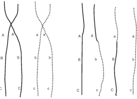
ABO blood gene is an example of a polymorphic locus. The set of alleles is (A, B, or O) with genotypes AA, AB, AO, etc. By haplotype, we mean a specific set of alleles on a person’s chromosome (7). We provide an example in Figure 1.

In the process of meiosis (the cell division that leads to the for-mation of egg or sperm cells), homologous chromosomes first pair up and then separate (7). In the process of separation, the homolo-gous chromosomes maintain 1 or more regions of contact known as chiasmata. At these regions, exchange of chromosomal mate-rial among the pair of chromosomes takes place. This exchange is referred to as a recombination. An example presented in Figure 1 represents a recombination taking place between the first locus (with alleles A and a) and the second locus (with alleles B and b). The resultant haplotypes (shown as strings of letters on the right-hand side) are: ABC, Abc, aBC, and abc.

The term recombination fraction refers to the probability that a recombination will take place between 2 loci. Theoretically, the range of the recombination fraction between 2 loci is 0–0.5. A recombination fraction of 0 means that no recombination ever takes place between the 2 loci and indicates that they are extremely close to one another on a chromosome. A 0.5 recombination frac-tion means that the loci are “unlinked.” For example, 2 loci on 2 different chromosomes have a recombination fraction of 0.5. Simi-larly, loci that are on opposite ends of a chromosome may have a recombination fraction very close to 0.5.

Statistical methods that estimate the recombination fraction between 2 loci using genotype data from families (usually with a disease of interest) are referred to as linkage methods. Such meth-ods have been highly successfully in finding disease genes for very rare diseases that act in a dominant or recessive fashion (8).

The term linkage disequilibrium (LD) refers to a nonrandom relationship between 2 alleles that typically arises because those alleles are closely linked on a chromosome and therefore infre-quently separated from one another by recombination. In this case, the frequency of each allele in the population does not allow one to predict the frequency at which they occur together. Typi-cally, one of the loci is an observed marker locus, and the other is

Nonstandard abbreviations used: HRR, haplotype relative risk; HWE, Hardy-Wein-berg equilibrium; IDDM, insulin-dependent diabetes mellitus; LD, linkage disequi-librium; MSSN, minimal sample size necessary; PDT, pedigree disequilibrium test; PL, power loss; Pr, probability; PSA, prostate-specific antigen; SNP, single nucleotide polymorphism; TDT, transmission disequilibrium test.

Conflict of interest: The authors have declared that no conflict of interest exists.

the disease locus. One of the common measures of LD is D′, a stan-dardized measure of LD (9), which ranges between 0 and 1. When 2 loci are completely unlinked (for example, if they are on different chromosomes), D′ = 0. If the 2 loci are identical (for example, a marker locus is the disease locus), then D′ = 1. Values of D′ closer to 1 suggest that the marker locus is closer to the disease locus. It has been shown that, under certain circumstances, statistical methods involving LD have a significantly higher probability of finding dis-ease genes than do linkage methods (5). Thus, LD methods are of critical importance in mapping disease loci.

By Hardy-Weinberg equilibrium (HWE), we mean that the gen-otype frequencies for a locus can be completely described by the allele frequencies. Here, the term frequency refers to the propor-tion of either an allele or a genotype in the populapropor-tion. As an exam-ple, suppose we have a diallelic SNP locus with alleles A and B. If the frequency of the A allele is pA and the frequency of the B allele

is pB, then, in the condition of HWE, the genotype frequencies for

AA, AB, and BB are pA2, 2pApB, and pB2, respectively.

Penetrance refers to the probability that an individual is affected if that individual has a certain genotype at the disease locus. For a diallelic disease locus, there will be 3 genotypes (having 0, 1, or 2 copies of the disease allele). Formally, fi = Pr(affected | i copies

of disease allele) (i = 0, 1, 2), where f indicates penetrance and Pr indicates probability. That is, f0 is the probability of being affected

in individuals who have 0 copies of the disease gene, f1 is the

prob-ability with 1 copy of the disease gene, f2 is the probability with 2

copies. Example penetrances for different diseases are: f0 = f1 = 0,

f2 = 1 for cystic fibrosis (10), a recessive disease, and f0 = 0.08,

f1 = 0.82, f2 = 0.82 for certain groups of patients with the BRCA1

mutation for breast cancer (11), a dominant disease. More gener-ally, recessive diseases are those for which f0 = f1, and dominant

diseases are those for which f1 = f2.

The term phenotype refers to an observed disease status. Exam-ple disease phenotypes are presence or absence of: diabetes, heart disease, colon cancer, breast cancer, male prostate cancer, psoriasis, Alzheimer disease, and schizophrenia. Typically, those who have the presence of a disease phenotype are called cases and those who have an absence of the disease phenotype are called controls.

We illustrate the concept of statistical power with an example. When an (unobserved) disease locus is situated near an (observed) marker locus, the genotype frequencies in individuals affected with the disease will differ from frequencies in individuals who are not affected with the disease. One statistical test designed to detect these differences is the Pearson χ2 _{test of independence. An example of its}

application is provided in Table 1. If the value of the test statistic is sufficiently large, then we correctly reject the null hypothesis that there is no association between the disease phenotype and the mark-er locus; that is, the test statistic indicates that the markmark-er locus is in the proximity of a disease locus. Thus, power is the probability that the test statistic indicates (usually when the statistic has a large value) that the observed marker loci are near an (unobserved) dis-ease locus. The concept of power is intimately related to the concept of type I error. The type I error rate is the probability that the test statistic indicates that the observed marker loci are near a disease locus when in fact there is no disease locus nearby. One controls the type I error by setting appropriate thresholds for the test statistic. If the value of the statistic for a data set (of marker locus genotypes) is below the threshold, then we accept the null hypothesis that there in no disease gene in the vicinity of the marker locus. Traditionally, we write this as accepting the null hypothesis that there is no association between the marker and the disease phenotype. The type I error rate and power of a study are the 2 key design parameters of a study.

Misclassification refers to either an observed phenotype or type that is different from the true underlying phenotype or geno-type, respectively. Historically, the term misclassification has been used in statistics (12, 13) to mean the same as phenotype or geno-type error in statistical genetics and genetics. Hereafter, we use the term error to mean misclassification in the statistical sense. An example of phenotype misclassification involves use of the pros-tate-specific antigen (PSA) test for diagnosis of male prostate can-cer (14). There may be a lack of PSA elevation in some men with prostate cancer, resulting in an affected individual (case) being misclassified as an unaffected individual (control). An example of genotype misclassification for a marker locus with genotypes AA, AB, and BB is a heterozygote individual (AB) being recorded as having either an AA or BB genotype (15).

Finally, for tests of association applied to contingency tables, we use the abbreviation PL to mean power loss for a fixed sample size and given type I error rate in the presence of errors; and the abbreviation MSSN to mean the minimal sample size necessary to maintain constant power for a given type I error rate. For example, suppose that we have collected data from 100 cases and 100 con-trols that we have genotyped at a diallelic SNP locus with alleles A and B. Suppose further that both case and control populations are in HWE before the introduction of genotype error and have A allele frequencies of 0.05 and 0.10, respectively. Furthermore, assume that any homozygote is randomly misclassified as the heterozygote with a 0.01 probability and similarly the heterozygote is randomly misclassified as either homozygote with a 0.01 prob-ability. Then the power to detect association using the χ2 _{test of}

independence (also see “Population-based association/Statistical methods” below) is 38% at the 5% type I error rate when no misclas-sification errors are present, and it is 35% when random errors are present, resulting in a PL of 0.376 – 0.353 = 0.023 (16, 17). That is,

Figure 1

the probability of detecting a nearby disease locus is reduced by 2.3%. Similarly, if we have the same genotype frequency settings in cases and controls and we wish to compute the MSSN to achieve 95% statistical power with equal numbers of cases and controls for the χ2 _{test on genotypes, then we require 432 cases and 432}

con-trols when no errors are present; and we require a minimal sample size of 463 cases and 463 controls when random genotype errors are present in the data. The presence of genotype errors results in a 7.26% increase in MSSN to maintain the same statistical power.

Other critical concepts that are basic to an understanding of sta-tistical methods for disease gene mapping are replication and mul-tiple testing. Often, statistical evidence for association may be due to chance. A way to eliminate chance as an explanation for the associa-tion is to replicate the findings in an independent data set (8). Another way that false positive findings can occur is through multiple testing. Suppose that we wish to test 2 markers, 1 on each end of every one of the human chromosomes with the exception of the sex chromosomes (a total of 22 chromosomes), for association with a given disease phe-notype. We would then conduct a total of 44 (2 × 22) independent tests. If we select a type I error rate of 5%, then the probability that at least 1 of the test statistics will reject the null hypothesis even when it is true can be shown to be approximately 88%. That means that, even if there is no disease gene in the entire genome, at least 1 marker would return a statistical test value suggesting the proximity of a dis-ease locus 88% of the time. There have been numerous proposals on how to correct for this inflation in type I error (18, 19).

Population-based association

Statistical methods

By population-based association, we refer to gene-mapping studies in which the data collected are for unrelated cases and controls. The data used to test for association are often presented in the form of contingency tables (20). The contingency tables for our purposes are ones in which rows describe an affection status (case or control) and the columns refer to either specific alleles, geno-types, or haplotypes (7, 21). An example of a contingency table for case and control individuals genotyped at a diallelic SNP locus is presented in Table 1. Let us assume that the individuals rep-resented in that table were categorized according to whether or not they have a disease such as breast cancer. A commonly used test statistic for association testing with such data is the χ2 _test

of independence. For the example data set we provide in Table 1, the value of the χ2 _{statistic is 8.17 with a corresponding P value of}

0.017. Because the P value is less than 0.05, based on the result, we

reject the null hypothesis of no association between colon cancer and this marker locus at the 5% type I error rate. In other words, this marker locus appears to be in close proximity to such a suscep-tibility locus for colon cancer based on these data.

Mitra (22) computed the noncentrality parameter of the asymp-totic distribution of the χ2 _{test on r×c contingency tables (r, rows;}

c, columns) for a specified alternative hypothesis. This noncentrality parameter is the key to computing power and sample size. It enables one to compute sample size requirements to guarantee a certain probability of detecting association at any given type I error rate

before any data are collected. In the example above, where we specified a power of 95% to detect association at the 5% type I error rate, we used Mitra’s formulation of the noncentrality parameter to deter-mine that we require a minimal sample size of 432 cases and 432 controls with errorless data. We performed this calculation using the Power for Association with Errors (PAWE) web tool (http://link-age.rockefeller.edu/pawe). Calculations such as these are critical for genetics researchers who wish to map susceptibility genes.

Family-based tests of linkage and association

Family-based methods of association were originally developed to address problems of population stratification in population-based methods of association. What is meant by population stratifica-tion? It is a phenomenon in which case individuals are drawn from one population and control individuals are drawn from another. For example, suppose we have a marker locus with alleles A and B that is completely unlinked to a disease locus (for example, it is on a different chromosome). Furthermore, suppose that the A allele fre-quency in white individuals is 0.5 and the A allele frefre-quency in Afri-can AmeriAfri-cans is 0.1. Because the marker locus is unlinked to the disease locus, we expect the A allele frequency to be 0.5 for both cases and controls in the white population and 0.1 for both cases and con-trols in the African American population. Therefore, if we draw 50 cases from the white population and 50 controls from the African American population, the χ2 _{test of independence will indicate the}

presence of a nearby disease locus with probability of 100% for a 5% type I error rate. That is, the statistic will always falsely indicate the presence of a disease locus, even though we have specified that we want the test statistic to only falsely reject the true null hypothesis 5% of the time. This is an example of Simpson’s paradox (23).

One of the problems with case-control studies is that control indi-viduals may not be well matched to cases, and thus association tests such as the χ2 _{test of association may provide false positive results}

for association (7). For example, if the control population is taken from hospital blood donors, then this sample may not be represen-tative of the population from which the case individuals are drawn, as hospital blood donors undergo more rigorous screening and are therefore considered to be “super-healthy” individuals (24).

Genomic control (25, 26) is one tool for dealing with this issue. Genomic control techniques use the markers from the genome to create appropriate corrections for population-based association tests. Other tools include statistical genetics methods that use fam-ily-based controls and that are robust to population stratification. The first such family-based method was the haplotype relative risk (HRR) method developed by Falk and Rubinstein (27–29).

Another method using family-based controls was developed by Spielman et al. (30) and is called the transmission disequilibrium test (TDT). The TDT focuses on transmitted and nontransmitted alleles from heterozygous parents to an affected offspring. The authors applied their method to data collected from 94 families

Table 1

Example contingency table for case and control individuals genotyped at a diallelic marker locus (hypothetical data)

Genotype

Affection status AA AB BB Row total

Case 23 47 30 100

Control 12 40 48 100 Column total 35 98 67 200

with 2 or more children with insulin-dependent diabetes mellitus (IDDM). The marker locus for which individuals were genotyped was the 5′ flanking polymorphism adjacent to the insulin gene on chromosome 11p (31). Their results showed that 1 allele (the class 1 allele) was transmitted 78 times from heterozygous parents to affect-ed offspring as opposaffect-ed to 42 times to unaffectaffect-ed offspring. The test statistic for these data was 11.5 with a corresponding P value of 0.0007, which suggests linkage between this locus and IDDM.

Spielman and Ewens later documented (32) that their test sta-tistic is valid even when multiple offspring from a pedigree are included, unlike the HRR methods, which inflate the type I error rate when multiple offspring are included. Because of the feature allowing for multiple offspring to be included, TDT methods have become very popular, and the original 1993 paper has been cited more than 1,600 times (according to the ISI Web of Science data-base). Examples where the TDT has been applied include studies of IDDM (30), psoriasis (33), Graves disease (34), schizophrenia (35), and many other diseases.

We illustrate the TDT calculation as follows. Phenotype and genotype data are collected on trios consisting of a father, mother, and an affected child. Consider a fully penetrant recessive disease with no phenocopies (i.e., the penetrances are: f0 = 0, f1 = 0, f2 = 1)

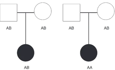
for which the disease locus is an SNP locus with 2 alleles desig-nated A (disease) and B (nondisease). Then the father and mother must have genotype AB and the affected child must have genotype AA at the SNP locus. Any such trio provides a value of 2 for the number of heterozygous parents who transmit an A allele to an affected child, more than the 1 expected under the null hypothesis of independent transmission. We also display this information pictorially in Figure 2. In this figure, we present the configuration of genotypes most likely to be observed under the null and alterna-tive hypotheses when the A allele frequency is 0.5. Note that under the null hypothesis, neither allele is preferentially transmitted to the affected child. Under the alternative hypothesis, the A allele is transmitted twice to the affected child.

In general, the TDT test detects an excess proportion of allele A transmissions to affected children. Among the extensions of the origi-nal TDT paper is a family-based method of association called the pedi-gree disequilibrium test (PDT), which is a valid test of association (i.e., does not increase type I error rate above the rate set by the researcher) even when multiple affected offspring from a pedigree are used (36). Other family-based tests of association that are valid for multiple affected siblings per family have also been developed (37, 38).

The TDT has limitations, however. The original statistic shows inflation in type I error rate where there is missing parental gen-otype information (39) or undetected gengen-otype errors (40, 41). Mitchell et al. (41) proved mathematically that ignoring undetect-ed genotype errors in the TDT can lead to substantial increases in the type I error rate of the original TDT. In particular, they showed that such a procedure can cause apparent transmission distortion at markers with alleles of unequal frequency and that this distor-tion is in the direcdistor-tion of indicating overtransmission of common alleles. Furthermore, they documented that in 79 published stud-ies that they investigated, the most common allele was reported to be overtransmitted to affected offspring in 31 (39%) of them. They concluded that undetected genotype errors may contribute to an inflated type I (that is, false positive) rate among reported TDT-derived findings. The exact extent and practical implications of these properties are ambiguous.

Finally, the original TDT is most powerful when a multiplicative relative risk model for the disease holds (42). That is, the increase in risk of affection for an individual having 2 copies of the disease allele is the square of the increase in risk of affection for having 1 copy of the disease allele [i.e., (f1 / f0)2 = f2 / f0]. One can see that this

is a restrictive assumption. For example, it does not hold true for dominant diseases, where the increase in risk is equal whether an individual has 1 or both copies of the disease allele. As a result, the original TDT may lose power to localize genes when the underly-ing disease inheritance is not multiplicative.

Extensions of the TDT method that allow for missing parental genotype information (43–45), genotype errors (40), and for more general disease models (45–47) have been developed. Recently, a TDT statistic that incorporates all 3 types of extensions has been developed (48). Software that performs the computations is pub-licly available (TDTae [transmission disequilibrium test allowing for errors]; ftp://linkage.rockefeller.edu/software/tdtae2/).

Factors affecting power

Disease allele frequency

While LD is often mentioned as a critical (if not the critical) factor with regard to power to detect association (4), an often overlooked factor is the difference between the disease allele frequency and the frequency of either the single SNP or haplotype that is in LD with the disease allele. It has been shown that in the TDT (49, 50) and case-control (51, 52) methods, power is a function of both LD between disease allele and the marker allele or haplotype and the difference of the disease allele frequency and the frequency of the marker allele or haplotype in LD with the disease allele. Power is maximal (or, equivalently, sample size is minimal) when the LD is maximal (e.g., Lewontin’s D′ = 1; ref. 9), and the frequency differ-ence is 0. Such a situation would occur, for example, if the marker allele were the disease allele.

Suppose that we consider cases and controls for Alzheimer disease, and the marker locus being considered is the apoE

Figure 2

locus on chromosome 19. For most populations, this locus has 3 alleles, designated ε2, ε3, and ε4. According to an

often-replicated finding, ε4 is the disease allele (53) with penetrances

approximately satisfying the equations f1 = 3 f0 and f2 = 32f0 = 9 f0.

That is, every additional copy of the ε4 allele produces an

approxi-mate 3-fold increase in an individual’s probability of becoming affected. Note that this disease inheritance model is multiplica-tive. Let us assume that the disease prevalence (that is, the prob-ability that a randomly selected individual from the population has the disease) is 0.012; the disease allele (ε4) frequency is 0.2;

the disease allele is in complete LD (D′ = 1) with an SNP marker locus allele A; the frequency of allele A is represented by pA; and

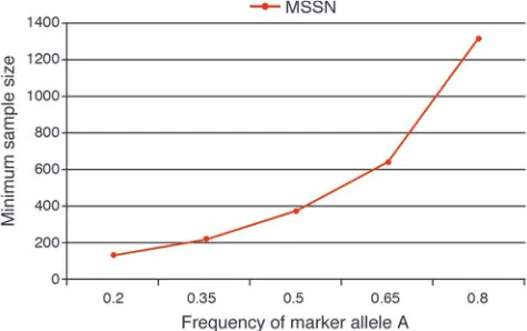
there are no phenotype or genotype errors. In Figure 3, we pro-vide minimal sample size requirements for power of 95% at the 5% type I error rate with Pearson’s χ2 _{test applied to 2 × 3}

con-tingency tables. These sample size calculations were determined using the PAWE web tool (http://linkage.rockefeller.edu/pawe/) by making the following selections: on the first page, Sample size calculations for a fixed power, Genetic model based method, Gor-don Heath Liu Ott error model, significance level = 0.05; on the second page, Power level between 0 and 1 = 0.95, Ratio of controls to cases = 1, Pr(affected | ++) = 0.0061, Pr(affected | +d) = 0.0184, Pr(affected | dd) = 0.0551, disease allele frequency = 0.2, SNP marker allele frequency = 0.2 to 0.8 in increments of 0.15, pro-portion of total disequilibrium D′ = 1, ε1 = 0.00001, ε2 = 0.00001

(error model parameters are not important, since we only look at results of data without error); on the third page, Data Without Error, Genotypic Test Results. Even when D′ = 1 between the dis-ease and the marker loci, we see a 10-fold incrdis-ease in MSSN when the SNP marker allele frequency is 0.8 compared with a frequency of 0.2 (the value of the disease allele frequency). This means that if we did not know the location of the ApoE gene and we typed SNP markers nearby the gene to test for association, our ability to detect association would depend heavily upon the SNP allele

frequency being in LD with apoEε4 allele. This result was actually

observed in a proof-of-principle study of association for Alzheim-er disease with SNP loci in or near the ApoE locus (54).

Genotype relative risk (effect size)

By genotype relative risk, we mean the ratios r1 = f1 / f0 and r2 = f2 / f0

(46). From a clinical perspective, the larger the genotype relative risk, the more easily one can distinguish an individual’s disease genotype based on their disease phenotype (presence or absence of a disease). The LOD score method (55) used in mapping genes for Mendelian traits has been highly successful (8). By Mendelian, we mean traits that follow either a dominant or recessive underly-ing disease inheritance and for which genotype relative risks are on the order of 1,000 or more. Examples of such traits include: cystic fibrosis (56–58), Huntington disease (59), breast cancer (11, 60), neurofibromatosis (61), and others (e.g., refs. 62–65).

Regarding complex (i.e., non-Mendelian) diseases, Page et al. (8) comment that there has been relatively little success “in the identi-fication of genes responsible for complex diseases.” Some notable exceptions are Crohn disease (66) and psoriasis (33, 67). What is it about the diseases in which genes have been identified that enables causative polymorphisms to be more readily discovered? To be sure, one key feature is that these diseases are not characterized by large phenotype error. We would suggest that another key feature is that the genotype relative risks for these diseases are sufficiently large so that association can be established with small to moderate (fewer than 500 cases and controls or fewer than 300 trios) sample sizes. In a recent Crohn disease study, Franchimont et al. (68) documented that carrying certain alleles in both genes TLR4 and NOD2 is associated with a genotype relative risk of 4.7. In other recent publications, highly significant evidence was found for both linkage (69) and association (67, 70) with psoriasis in HLA region of chromosome 6. In the case of association, the statistical analyses were performed with trio (father, mother, affected offspring) and case-control designs with genotype relative risks estimated to be over 100. The interpretation is that if an individual has at least 1 copy of the disease allele for psoriasis, the probability that he or she will show the phenotype is at least 100 times the probability for a person without a copy of the disease allele.

Misclassification error

An often-overlooked factor in determining whether genes can be detected using association testing is the presence of pheno-type and/or genopheno-type misclassification error (71). Such errors are important because without some method of adjustment, the power to detect association and thus to map genes may be signifi-cantly decreased (16, 72).

Breslow and Day (21) attribute the first statistical work on errors in association tests applied to contingency tables to Bross (72). In his work, Bross (72) focused on the χ2 _{test of independence applied}

to 2 × 2 contingency tables and what we term phenotype error, namely the effects of misclassifying a case subject as a control and vice versa. Bross found that there is no change in the level of sig-nificance (i.e., the type I error rate remains constant), the power for the χ2 _{test is reduced, and estimates of the proportions of cases}

and controls are biased away from their true values. For example, if the true proportions of cases and controls were each 0.50, in the presence of phenotype error, one might estimate proportions of 0.6 and 0.4 for cases and controls, respectively.

Mote and Anderson (73) proved mathematically that the power of the χ2 _{test with no error is always greater than or equal to the power}

Figure 3

Minimum sample size requirement (cases and controls) for case-con-trol design for different values of SNP marker allele frequency. This figure provides the minimum number of cases and controls assum-ing the followassum-ing genetic model parameters: f0 = 0.0061, f1 = 0.0184,

f2 = 0.0551, pd = 0.2, and LD measure D′ = 1 between disease allele and marker allele A. Note that the penetrances satisfy the equations:

of the test when errors are present and ignored. Sturmer et al. (74) point out that correction for error is rarely carried out in practice, particularly for case-control designs. One explanation these authors provide for this phenomenon is that appropriate software is not available. More specifically, methods incorporating misclassifica-tion error have not been applied to genetic associamisclassifica-tion studies with actual phenotype, genotype, or haplotype data. The implications are that researchers trying to map complex-trait genes will not know by how much they are underestimating their statistical power in the presence of error. Thus, for example, a study that would have 95% power to detect association based on a sample size of 100 observed cases and 100 observed controls provided that there were not phe-notype errors, may in fact only have 85% power when 10% of the cases have been misclassified as controls and vice versa.

Phenotype error

Phenotype error is a principal concern in many epidemiology studies. Thomas et al. (75), Gustafson (76), and others provide an overview of issues and techniques (77–81). These works all deal with environmental as opposed to genetic association. Also, the problem of the “cost” of errors (that is, the percent increase in sam-ple size necessary to maintain constant power in the presence of errors) has not been treated in these studies (see “What SNP geno-type errors require largest minimal sample size” below). What are examples of phenotype error? One example comes from the study of Alzheimer disease. Some researchers may use clinical dementia tests as a means of diagnosing Alzheimer disease (82, 83). However, not all individuals who show clinical dementia necessarily develop Alzheimer disease (82). Another example of phenotype error is the one previously mentioned: use of the PSA test for diagnosis of male prostate cancer (14). There may be a lack of PSA elevation in some men with prostate cancer, resulting in an affected individual (case) being misclassified as an unaffected individual (control).

Arguably the most frequently documented form of phenotype error for Mendelian genetic traits is locus heterogeneity (7). By this we mean that individuals in different pedigrees may have phenotypi-cally indistinguishable forms of a disease but show the phenotype due to mutations in different genes in the genome. For nonsyn-dromic hearing loss alone, more than 100 genes have been estab-lished by linkage (84), and each mutation leads to the same phe-notype. Biologically, the explanation for locus heterogeneity is that any gene in a pathway being disrupted can result in the disease

phe-notype. Among the most well-known examples of diseases display-ing locus heterogeneity are breast cancer (11), prostate cancer (85), nonsyndromic hearing loss (84), and macular degeneration (86).

Genotype errors in linkage and association studies

A number of authors have looked at the effects of genotype errors on linkage and association studies (13, 40, 87–95). Sobel et al. (6) provide a thorough summary. Gordon, Finch, et al. (16, 17) quan-tified the loss in power for case-control studies of genetic associa-tion due to genotype errors. Specifically, they calculated the effects that errors in genotype have on power and MSSN to maintain con-stant type I error and power, using 3 published models of genotype errors on the χ2 _{test for independence in the 2 × 3 table. The PAWE}

website performs power and sample size calculations for genetic association analysis with case-control data based on this work.

For an example of the effects of genotype errors, consider the data in Table 1, representing 100 cases and 100 controls genotyped at a diallelic locus with alleles A and B. The data in Table 1 are without genotype error, and the probability of misclassifying a homozygote (either AA or AB) as the heterozygote AB is 10%; similarly, the ability of misclassifying AB as either AA or BB is 10% with 0% prob-ability of misclassifying AA as BB or vice versa. Thus on average we would expect the genotype counts to change as follows: 10% of the 23 AA genotypes (i.e., 2.3 on average) in cases would be misclassi-fied as AB, and 10% of the 47 AB genotypes (i.e., 4.7 on average) in cases would be misclassified as AA genotypes, with the resultant effect of 4.7 – 2.3 ≈ 2 additional “observed” AA genotypes expected in cases, bringing the number to 25 “observed” AA genotypes in cases when genotype errors are present. Similarly, 4.7 of the AB genotypes on average would be misclassified as BB genotypes in cases, and 3 of the 30 BB genotypes on average in cases (10%) would be misclassified as AB genotypes, with a result of 4.7 – 2.3 ≈ 2 addi-tional “observed” genotypes expected in cases with BB genotype, giving a total of 32 “observed” case BB genotypes in the presence of errors. The calculations were performed for all genotypes in Table 1, and the results are shown in Table 2. If we apply the χ2 _{test to the}

data counts in Table 2, the test statistic is 5.66, with a correspond-ing P value of 0.059. In other words, with these errors, our data set has gone from being significant to not being significant (at the 5% type I error rate). So, we may “miss” the signal.

Another approach to performing association analyses with cases and controls involves the pooling of multiple individuals’ geno-types to estimate allele frequencies. This technique is known as DNA pooling. Its primary advantage is a reduction in the cost of genotyping (96). As with techniques that involve individual geno-type counts, DNA pooling technologies are subject to misclassifi-cation error. Recently, Zou and Zhao (97) have looked at the effects of genotype errors on the power of case-control association stud-ies. These authors found that the majority of the positive findings from DNA pooling analyses may be false positives if measurement errors are not appropriately considered in the study design.

Statistical methods that detect or incorporate phenotype and/or genotype error

While there has been a significant amount of methodological work on statistical methods for association when data are misclassified (see “Misclassification error” above), there have been relatively few methods designed for the express purpose of association testing in a case-control design (98–103). Software is available only for the method described in ref. 103.

Table 2

Example contingency table for case and control individuals genotyped at a diallelic marker locus after genotype errors are introduced (hypothetical data)

Genotype

Affection status AA AB BB Row total

Case 25 43 32 100

Control 15 38 47 100 Column total 40 81 79 200

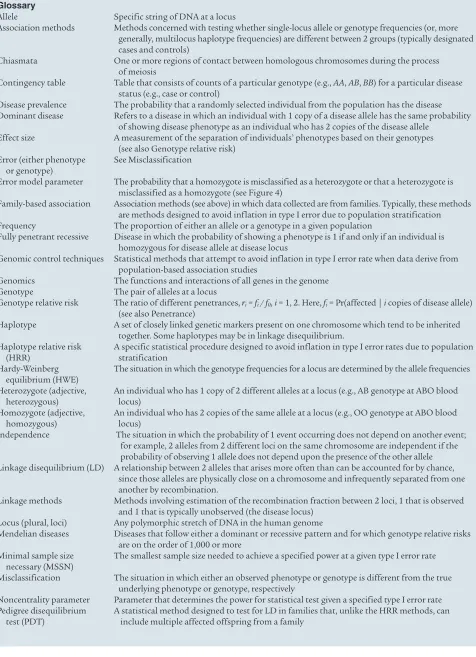
Glossary

Allele Specific string of DNA at a locus

Association methods Methods concerned with testing whether single-locus allele or genotype frequencies (or, more generally, multilocus haplotype frequencies) are different between 2 groups (typically designated cases and controls)

Chiasmata One or more regions of contact between homologous chromosomes during the process of meiosis

Contingency table Table that consists of counts of a particular genotype (e.g., AA, AB, BB) for a particular disease status (e.g., case or control)

Disease prevalence The probability that a randomly selected individual from the population has the disease Dominant disease Refers to a disease in which an individual with 1 copy of a disease allele has the same probability

of showing disease phenotype as an individual who has 2 copies of the disease allele Effect size A measurement of the separation of individuals’ phenotypes based on their genotypes

(see also Genotype relative risk) Error (either phenotype See Misclassification

or genotype)

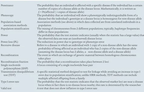
Error model parameter The probability that a homozygote is misclassified as a heterozygote or that a heterozygote is misclassified as a homozygote (see Figure 4)

Family-based association Association methods (see above) in which data collected are from families. Typically, these methods are methods designed to avoid inflation in type I error due to population stratification Frequency The proportion of either an allele or a genotype in a given population

Fully penetrant recessive Disease in which the probability of showing a phenotype is 1 if and only if an individual is homozygous for disease allele at disease locus

Genomic control techniques Statistical methods that attempt to avoid inflation in type I error rate when data derive from population-based association studies

Genomics The functions and interactions of all genes in the genome Genotype The pair of alleles at a locus

Genotype relative risk The ratio of different penetrances, ri = fi / f0, i = 1, 2. Here, fi = Pr(affected | i copies of disease allele)

(see also Penetrance)

Haplotype A set of closely linked genetic markers present on one chromosome which tend to be inherited together. Some haplotypes may be in linkage disequilibrium.

Haplotype relative risk A specific statistical procedure designed to avoid inflation in type I error rates due to population (HRR) stratification

Hardy-Weinberg The situation in which the genotype frequencies for a locus are determined by the allele frequencies equilibrium (HWE)

Heterozygote (adjective, An individual who has 1 copy of 2 different alleles at a locus (e.g., AB genotype at ABO blood heterozygous) locus)

Homozygote (adjective, An individual who has 2 copies of the same allele at a locus (e.g., OO genotype at ABO blood homozygous) locus)

Independence The situation in which the probability of 1 event occurring does not depend on another event; for example, 2 alleles from 2 different loci on the same chromosome are independent if the probability of observing 1 allele does not depend upon the presence of the other allele Linkage disequilibrium (LD) A relationship between 2 alleles that arises more often than can be accounted for by chance,

since those alleles are physically close on a chromosome and infrequently separated from one another by recombination.

Linkage methods Methods involving estimation of the recombination fraction between 2 loci, 1 that is observed and 1 that is typically unobserved (the disease locus)

Locus (plural, loci) Any polymorphic stretch of DNA in the human genome

Mendelian diseases Diseases that follow either a dominant or recessive pattern and for which genotype relative risks are on the order of 1,000 or more

Minimal sample size The smallest sample size needed to achieve a specified power at a given type I error rate necessary (MSSN)

Misclassification The situation in which either an observed phenotype or genotype is different from the true underlying phenotype or genotype, respectively

Regarding genotype error, much work has been done on the

detection of genotype errors in linkage and association studies (6, 87, 104–115). Recently, however, there has been work on the devel-opment of methods that incorporate genotype errors explicitly into the statistical methodology for family-based linkage studies (6, 103, 116–118), TDT (40), and case-control genetic association tests (101, 102). Two noteworthy contributions for TDT include the work by Bernardinelli et al. (119) and Morris and Kaplan (120). Both groups of authors develop statistics that are valid for linkage in the presence of association when either genotype errors are pres-ent or parpres-ental genotypes are missing (or both). Their methods are currently applicable only to trios (father, mother, affected child).

What SNP genotype errors require the largest minimal sample size?

Some recent work on the MSSN for genotype errors in case-con-trol studies indicates that misclassifying a more common genotype as a less common genotype requires a greater minimal sample size than the reverse misclassification (121, 122). In particular, Kang et al. (121) document that, as the control SNP minor allele frequen-cy approaches 0, the MSSN for misclassifying the more common homozygote as the less common homozygote and for misclassify-ing the heterozygote as the less common homozygote both increase without bound. These results suggest that researchers should take special care when scoring less common homozygotes. The implica-tions of this, as we have mentioned above, is that the probability of localizing disease genes is decreased. Consider the example of the fully penetrant recessive disease with no phenocopies we provided above (see “Family-based tests of linkage and association”), where the A allele is the disease allele and the B allele is the non-disease allele. If the disease is rare, then we expect that the A allele frequency is very small, and consequently the B allele frequency is large. If there

is no genotype error in the data, then only those individuals who are homozygous for the A allele will be affected, and intuitively, we will detect that locus relatively easily. Imagine now that we randomly misclassify the more common homozygote BB as the less common homozygote. Then we may observe unaffected individuals who also show the AA genotype, thus diluting the effect of the signal.

Designing association studies that are robust to errors

At this point, we hope it is clear that the effects of errors are to decrease the probability of finding disease genes and in some situations (e.g., family-based tests of association) to increase the false-positive rate, thereby increasing the probability of following up with studies on regions of the genome that do not harbor any genes for a disease of interest.

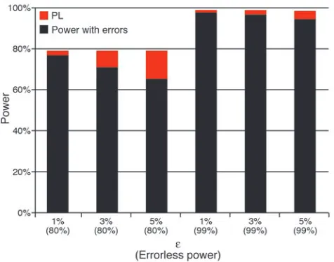
What can be done to address the issue of errors at the design stage, before any phenotypes are measured or genotyped scored? We believe the simplest answer to that question is: design the study to have higher power. We provide an illustration of this point in Figure 4, which shows the results of computation of statisti-cal power for the χ2 _{test of independence on 2 × 3 contingency}

tables (case patients and control individuals genotyped for a SNP marker locus) in the presence of genotype errors. Power is com-puted as a function of power without errors (2 settings for power are used: 99% and 80%) and an error model parameter ε. This parameter is the probability that a homozygote is misclassified as a heterozygote and the probability that a heterozygote is misclas-sified as a homozygote. It is assumed that homozygotes are not misclassified as other homozygotes (113). We consider 3 settings for the parameter ε: 1%, 3%, and 5%. Genotype frequencies for cases and controls are computed assuming the following genetic model parameters: f0 = 0.01, f1 = f2 = 0.02, pd = p1 = 0.1, D′ = 1.0.

Penetrance The probability that an individual is affected with a specific disease if the individual has a certain number of copies of a disease allele at the disease locus. Mathematically, it is written as

fi = Pr(affected | i copies of disease allele)

Phenocopy The probability that an individual will show a phenotypically indistinguishable form of a disease but the individual’s genotype at a disease locus is homozygous for non-disease allele Population-based Association methods (see above) in which data collected are from unrelated individuals in a association methods population

Population stratification The mixing of chromosomes from 2 different populations; typically, haplotype frequencies differ in these populations

Power The probability that the test statistic indicates (usually when the statistic has a large value) that the observed data are near an (unobserved) disease locus

Power loss (PL) The reduction in power due to genotype or phenotype error

Recessive disease Refers to a disease in which an individual with 1 copy of a non-disease allele has the same probability of being affected as an individual who has 2 copies of the non-disease allele (assuming the disease locus has 2 alleles, a non-disease allele and a disease allele) Recombination The event in which an exchange of genetic material between homologous chromosomes

takes place

Recombination fraction The probability that a recombination takes place between 2 loci Single nucleotide A locus consisting of a single nucleotide base pair

polymorphism (SNP)

Transmission disequilibrium A specific statistical method designed to test for linkage while avoiding an increase in type I test (TDT) error due to population stratification; unlike HRR methods, TDT methods can include

multiple affected offspring from a family

That is, we assume a dominant underlying disease inheritance for the disease where the SNP marker locus is the disease locus. The notation pd and p1 refer to the disease allele frequency and

marker locus minor allele frequency, respectively. For a power of 99%, a minimum of 606 case patients and 606 control individu-als are required, assuming equal numbers of cases and controls. Similarly, for a power of 80%, a minimum of 307 case patients and 307 control individuals are required. PL, which is the differ-ence of the power without errors and the power in the presdiffer-ence of errors, is represented graphically as the red portion of each bar. All power values were computed using the PAWE web tool (http://linkage.rockefeller.edu/pawe/). These power values were achieved by making the following selections: on the first page, Power calculations for a fixed sample size, Genetic model based method, Sobel Papp Lange error model, Significance level = 0.01; on the second page, Number of case individuals = Number of control individuals = 606 (99% power level) or 307 (80% power level), Pr(affected | ++) = 0.01, Pr(affected | +d) = 0.02, Pr(affected | dd) = 0.02, disease allele frequency = 0.1, SNP marker allele fre-quency = 0.1, proportion of total disequilibrium D′ = 1, V1 = ε,

V2 = 0.000001, V3 = ε (ε = 0.01, 0.03, or 0.05); on the third page,

Data Without Error, Genotypic Test Results, Data With Error, Genotypic Test Results, Power Loss.

The PL when power without errors is 99% is always less than the corresponding PL (for a given value ε) when power without errors is 80%. In fact, the PL for the 99% settings is no more than one-fourth of the PL for the 80% settings, as in the example where

ε = 5%. In that instance, PL for the 99% settings is 3.5%, as com-pared with a loss of 14.6% for the 80% setting. This means that if we designed our study to have power of 99%, then we would still have 95.5% power after errors, whereas if we designed our study to have power of 80%, we would only have power of 65.4% after errors. This example demonstrates the added advantage of robustness to misclassification error when high power is specified at the design stage of an association study. In other words, by specifying a power of 99% and “paying the cost up front” by collecting 606 each of case patients and controls, we reduce the effect of genotype errors on the power of the χ2 _{test, as compared with the PL that would}

occur if we only designed our study to have 80% power and only collected 307 each of case patients and controls.

Conclusions

Here, we reviewed family-based and population-based methods for association, specified the factors that determine power, and showed that study design and analysis should examine a range of settings of the important factors. The factors we discussed include: the disease allele frequency or, more specifically, the difference of the disease allele frequency and the marker allele or haplotype fre-quency in LD with the disease allele; genotype relative risk (effect size); and phenotype and genotype misclassification error rates. We focused on this third factor because it is commonly overlooked when the power to detect association is computed, even though random misclassification error always reduces power (73).

For TDT methods, random misclassification errors lead to an increase in the type I error rate of the test statistic, which may be an even more important problem than loss of power to detect associa-tion. The TDTae method avoids this problem (40, 48).

To reduce costs and to increase the accuracy of association stud-ies, it is vitally important to develop methods that either incorpo-rate errors into the analysis or that quantify the effects of errors (in terms of PL or MSSN for different statistical tests). Developing statistical methods that achieve maximal power and correct type I error rates in the presence of errors saves researchers time and money, either by providing the researchers with statistical meth-ods with sufficient power to detect associations even in the pres-ence of errors or by protecting the researchers from finding and following up on false positive results in the genome.

Finally, what is a simple procedure to help insure that genetic asso-ciation studies will be more robust to error? We recommend specify-ing higher power values when computspecify-ing sample size requirements.

Acknowledgments

The authors gratefully acknowledge grants K01-HG00055 and MH44292 from the NIH. The authors also gratefully acknowledge A. Bowcock, who provided useful information on phenotyping issues relating to psoriasis.

Address correspondence to: Derek Gordon, Laboratory of Statisti-cal Genetics, Rockefeller University, Box 192, 1230 York Avenue, New York, New York 10021, USA. Phone: (212) 327-7987; Fax: (212) 327-7996; E-mail: [email protected].

Figure 4

Power loss (PL) for genetic association as a function of errorless power threshold and error probability ε. In this figure, we compute statistical power for the χ2 _{test of independence on 2 × 3 contingency tables in} the presence of genotype errors. Power is computed as a function of power without errors (2 settings for power used: 99% and 80%) and an error model parameter ε. This parameter is the probability that a homozygote is misclassified as a heterozygote and the probability that a heterozygote is misclassified as a homozygote. It is assumed that homozygotes are not misclassified as other homozygotes (113). We consider 3 settings for the parameter ε: 1%, 3%, and 5%. Each bar rep-resents 2 values: power in the presence of errors (black portion of each bar) and PL, which is the difference of the power without errors and the power in the presence of errors (represented graphically as the red portion of each bar). Genotype frequencies for cases and controls are computed assuming the following genetic model parameters: f0 = 0.01,

1. Lander, E.S., et al. 2001. Initial sequencing and anal-ysis of the human genome. Nature.409:860–921. 2. Venter, J.C., et al. 2001. The sequence of the human

genome. Science.291:1304–1351.

3. Guttmacher, A.E., and Collins, F.S. 2002. Genomic medicine — a primer. N. Engl. J. Med.347:1512–1520. 4. Gabriel, S.B., et al. 2002. The structure of

haplotype blocks in the human genome. Science. 296:2225–2229.

5. Risch, N., and Merikangas, K. 1996. The future of genetic studies of complex human diseases. Science. 273:1516–1517.

6. Sobel, E., Papp, J.C., and Lange, K. 2002. Detection and integration of genotyping errors in statistical genetics. Am. J. Hum. Genet.70:496–508. 7. Ott, J. 1999. Analysis of human genetic linkage. 3rd

edition. The Johns Hopkins University Press. Bal-timore, Maryland, USA. 405 pp.

8. Page, G.P., George, V., Go, R.C., Page, P.Z., and Alli-son, D.B. 2003. “Are we there yet?”: deciding when one has demonstrated specific genetic causation in complex diseases and quantitative traits. Am. J. Hum. Genet.73:711–719.

9. Lewontin, R.C. 1964. The interaction of selection and linkage. I. General considerations; heterotic models. Genetics.49:49–67.

10. Collins, F.S., Riordan, J.R., and Tsui, L.C. 1990. The cystic fibrosis gene: isolation and significance.

Hosp. Pract. (Off. Ed.).25:47–57.

11. Newman, B., Austin, M.A., Lee, M., and King, M.C. 1988. Inheritance of human breast cancer: evidence for autosomal dominant transmission in high-risk families. Proc. Natl. Acad. Sci. U. S. A.85:3044–3048. 12. Cochran, W.G. 1968. Errors of measurement in

sta-tistics. Technometrics.10:637–666.

13. Ott, J. 1977. Linkage analysis with misclassification at one locus. Clin. Genet.12:119–124.

14. Platz, E.A., De Marzo, A.M., and Giovannucci, E. 2004. Prostate cancer association studies: pitfalls and solutions to cancer misclassification in the PSA era. J. Cell. Biochem.91:553–571.

15. Miller, C.R., Joyce, P., and Waits, L.P. 2002. Assess-ing allelic dropout and genotype reliability usAssess-ing maximum likelihood. Genetics.160:357–366. 16. Gordon, D., Finch, S.J., Nothnagel, M., and Ott,

J. 2002. Power and sample size calculations for case-control genetic association tests when errors are present: application to single nucleotide polymorphisms. Hum. Hered.54:22–33.

17. Gordon, D., Levenstien, M.A., Finch, S.J., and Ott, J. 2003. Errors and linkage disequilibrium interact multiplicatively when computing sample sizes for genetic case-control association studies. Pac. Symp. Biocomput.2003:490–501.

18. Westfall, P.H., and Young, S.S. 1993. Resampling-based multiple testing. Wiley. New York,New York, USA. 360 pp.

19. Wille, A., Hoh, J., and Ott, J. 2003. Sum statistics for the joint detection of multiple disease loci in case-control association studies with SNP markers.

Genet. Epidemiol.25:350–359.

20. Fienberg, S.E. 1980. The analysis of cross-classified cat-egorical data. The MIT Press. Cambridge, Massachu-setts, USA. 224 pp.

21. Breslow, N.E., and Day, N.E. 1980. Statistical meth-ods in cancer research. The analysis of case-control studes. IARC Sci. Publ. 1:350.

22. Mitra, S.K. 1958. On the limiting power function of the frequency chi-square test. Ann. Math. Stat. 29:1221–1233.

23. Simpson, E.H. 1951. The interpretation of interac-tion in contingency tables. J. R. Stat. Soc.13:238–241. 24. Vineis, P., and McMichael, A.J. 1998. Bias and con-founding in molecular epidemiological studies: spe-cial considerations. Carcinogenesis.19:2063–2067. 25. Hoh, J., and Ott, J. 2004. Genetic dissection of

dis-eases: design and methods. Curr. Opin. Genet. Dev. 14:229–232.

26. Devlin, B., and Roeder, K. 1999. Genomic control for association studies. Biometrics.55:997–1004. 27. Falk, C.T., and Rubinstein, P. 1987. Haplotype

rela-tive risks: an easy reliable way to construct a proper control sample for risk calculations. Ann. Hum. Genet.51:227–233.

28. Ott, J. 1989. Statistical properties of the haplotype relative risk. Genet. Epidemiol.6:127–130. 29. Terwilliger, J.D., and Ott, J. 1992. A

haplotype-based ‘haplotype relative risk’ approach to detect-ing allelic associations. Hum. Hered.42:337–346. 30. Spielman, R.S., McGinnis, R.E., and Ewens, W.J.

1993. Transmission test for linkage disequilib-rium: the insulin gene region and insulin-depen-dent diabetes mellitus (IDDM). Am. J. Hum. Genet. 52:506–516.

31. Bell, G.I., Horita, S., and Karam, J.H. 1984. A poly-morphic locus near the human insulin gene is associated with insulin-dependent diabetes mel-litus. Diabetes.33:176–183.

32. Spielman, R.S., and Ewens, W.J. 1996. The TDT and other family-based tests for linkage disequilibrium and association. Am. J. Hum. Genet.59:983–989. 33. Helms, C., et al. 2003. A putative RUNX1 binding

site variant between SLC9A3R1 and NAT9 is asso-ciated with susceptibility to psoriasis. Nat. Genet. 35:349–356.

34. Chistiakov, D.A., Savost’anov, K.V., and Turaku-lov, R.I. 2004. Screening of SNPs at 18 positional candidate genes, located within the GD-1 locus on chromosome 14q23-q32, for susceptibility to Graves’ disease: a TDT study. Mol. Genet. Metab. 83:264–270.

35. Addington, A.M., et al. 2004. GAD1 (2q31.1), which encodes glutamic acid decarboxylase (GAD(67)), is associated with childhood-onset schizophrenia and cortical gray matter volume loss. Mol. Psychia-try. doi:10.1038/sj.mp.4001599.

36. Martin, E.R., Kaplan, N.L., and Weir, B.S. 1997. Tests for linkage and association in nuclear fami-lies. Am. J. Hum. Genet.61:439–448.

37. Horvath, S., Xu, X., and Laird, N.M. 2001. The family based association test method: strategies for studying general genotype — phenotype asso-ciations. Eur. J. Hum. Genet.9:301–306.

38. Liu, X., and Gordon, D. 2003. A general class of association tests for family-based data using weight functions. Genet. Epidemiol.24:208–219. 39. Curtis, D., and Sham, P.C. 1995. A note on the

application of the transmission disequilibrium test when a parent is missing. Am. J. Hum. Genet. 56:811–812.

40. Gordon, D., Heath, S.C., Liu, X., and Ott, J. 2001. A transmission/disequilibrium test that allows for genotyping errors in the analysis of single-nucleotide polymorphism data. Am. J. Hum. Genet. 69:371–380.

41. Mitchell, A.A., Cutler, D.J., and Chakravarti, A. 2003. Undetected genotyping errors cause appar-ent overtransmission of common alleles in the transmission/disequilibrium test. Am. J. Hum. Genet.72:598–610.

42. Clayton, D. 1999. A generalization of the transmis-sion/disequilibrium test for uncertain-haplotype transmission. Am. J. Hum. Genet.65:1170–1177. 43. Sun, F., Flanders, W.D., Yang, Q., and Khoury, M.J.

1999. Transmission disequilibrium test (TDT) when only one parent is available: the 1-TDT. Am. J. Epidemiol. 150:97–104.

44. Lee, W.C. 2002. Transmission/disequilibrium test when neither parent is available in some families: a non-iterative approach. J. Cancer Epidemiol. Prev. 7:97–103.

45. Weinberg, C.R. 1999. Allowing for missing parents in genetic studies of case-parent triads. Am. J. Hum. Genet.64:1186–1193.

46. Schaid, D.J., and Sommer, S.S. 1993. Genotype relative risks: methods for design and analysis of

candidate-gene association studies. Am. J. Hum. Genet.53:1114–1126.

47. Schaid, D.J. 1996. General score tests for associa-tions of genetic markers with disease using cases and their parents. Genet. Epidemiol.13:423–449. 48. Gordon, D., et al. 2004. A transmission

disequi-librium test for general pedigrees that is robust to the presence of random genotyping errors and any number of untyped parents. Eur. J. Hum. Genet. 12:752–761.

49. Abel, L., and Muller-Myhsok, B. 1998. Maximum-likelihood expression of the transmission/disequi-librium test and power considerations. Am. J. Hum. Genet.63:664–667.

50. Tu, I.P., and Whittemore, A.S. 1999. Power of asso-ciation and linkage tests when the disease alleles are unobserved. Am. J. Hum. Genet.64:641–649. 51. Zondervan, K.T., and Cardon, L.R. 2004. The

com-plex interplay among factors that influence allelic association. Nat. Rev. Genet.5:89–100.

52. Pfeiffer, R.M., and Gail, M.H. 2003. Sample size calculations for population- and family-based case-control association studies on marker genotypes.

Genet. Epidemiol. 25:136–148.

53. Corder, E.H., et al. 1993. Gene dose of apo-lipoprotein E type 4 allele and the risk of Alzheimer’s disease in late onset families. Science. 261:921–923.

54. Martin, E.R., et al. 2000. SNPing away at com-plex diseases: analysis of single-nucleotide polymorphisms around APOE in Alzheimer dis-ease. Am. J. Hum. Genet.67:383–394.

55. Morton, N.E. 1955. Sequential tests for the detec-tion linkage. Am. J. Hum. Genet. 7:277–318. 56. Rommens, J.M., et al. 1989. Physical localization of

two DNA markers closely linked to the cystic fibro-sis locus by pulsed-field gel electrophorefibro-sis. Am. J. Hum. Genet.45:932–941.

57. Kerem, B., et al. 1989. Identification of the cystic fibro-sis gene: genetic analyfibro-sis. Science.245:1073–1080. 58. Riordan, J.R., et al. 1989. Identification of the

cys-tic fibrosis gene: cloning and characterization of complementary DNA. Science.245:1066–1073. 59. The Huntington’s Disease Collaborative Research

Group. 1993. A novel gene containing a trinucleo-tide repeat that is expanded and unstable on Hun-tington’s disease chromosomes. Cell.72:971–983. 60. Futreal, P.A., et al. 1994. BRCA1 mutations in

primary breast and ovarian carcinomas. Science. 266:120–122.

61. Wallace, M.R., et al. 1991. A de novo Alu inser-tion results in neurofibromatosis type 1. Nature. 353:864–866.

62. Martinez-Mir, A., et al. 2003. Germline fumarate hydratase mutations in families with multiple cuta-neous and uterine leiomyomata. J. Invest. Dermatol. 121:741–744.

63. Martinez-Mir, A., et al. 2002. Multiple cutaneous and uterine leiomyomas: refinement of the genetic locus for multiple cutaneous and uterine leiomyo-mas on chromosome 1q42.3-43. J. Invest. Dermatol. 118:876–880.

64. Martinez-Mir, A., et al. 2002. EB simplex superfi-cialis resulting from a mutation in the type VII col-lagen gene. J. Invest. Dermatol.118:547–549. 65. Martinez-Mir, A., et al. 2003. Identification

of a locus for type I punctate palmoplantar keratoderma on chromosome 15q22-q24. J. Med. Genet.40:872–878.

66. Hugot, J.P., et al. 1996. Mapping of a susceptibil-ity locus for Crohn’s disease on chromosome 16.

Nature.379:821–823.

67. Veal, C.D., et al. 2002. Family-based analysis using a dense single-nucleotide polymorphism-based map defines genetic variation at PSORS1, the major psoriasis-susceptibility locus. Am. J. Hum. Genet. 71:554–564.