GEOGRAPHIC RELAY REGION BASED POWER AWARE
ROUTING IN WIRELESS SENSOR NETWORKS
1M. VIJU PRAKASH, 2B. PARAMASIVAN
1
Research Scholar, Manonmanium Sundaranar University, Tirunelveli, INDIA. 2
Professor and Head, National Engineering College, Kovilpatti, INDIA.
E-mail: [email protected] , [email protected]
ABSTRACT
Power aware routing is a powerful localized routing scheme for wireless sensor networks (WSNs) due to its scalability and efficiency. Maintaining neighborhood information for packet forwarding may not be suitable for WSNs in highly dynamic scenarios. Beacon-based protocols are maintaining neighbor information but does not comply on energy efficiency. We propose a novel routing scheme, called Geographic Relay Region based Power Aware Routing (GRRR), which can provide energy efficient, loop-free, stateless, sensor-to-sink power aware routing without the help of prior neighborhood information. In this routing scheme, each node first announces its next-hop optimum relay position on the straight line toward the sink and each node computes its quality value based on the residual power and distance between the optimum relay regions. Forwarder node is elected by the source based on quality value communicated using Request-To-Send/Clear-To-Send (RTS/CTS) handshaking mechanism. We establish the conditions for guaranteed delivery for sensor-to-sink routing, assuming no packet loss and no failures in greedy forwarding. We extend this scheme to lossy sensor networks to provide stable and efficient routing in the presence of unreliable communication links. Simulation results show that GRRR outperforms existing protocols with highly dynamic network topologies.
Keywords: Wireless Sensor Networks, Power-Aware Geographic Routing, Optimum Search Relay Region, Lossy Sensor Networks.
1. INTRODUCTION
The organized system of IEEE 802.15.4 contains low power micro-sensors and low-power RF design which can be connected wirelessly [1] [2] [3] to form a wireless sensor network. Geographic routing, in which each sensor node forwards packets only based on the locations of itself, its intended neighbors, and the target is particularly attractive to resource-constrained sensor networks. The nature of geographic routing reduces the overhead brought by route establishment and maintenance, signifying the advantages of modest memory requirement at each node and highly scalability in large network applications. In the conventional routing schemes, each node is required to maintain position information of all its neighbors, and the position of a node is made available to its direct neighbors by broadcasting beacons. In WSNs with invariant
network topology, maintaining neighborhood
information can greatly improve the performance, because of the reusability of the maintained information and minimal maintenance cost. However, in highly dynamic scenarios, network
topology may change frequently due to node mobility, sleeping [4] [5], link faults etc. In dynamic nature, maintaining neighbor information suffers from three factors. First, communication overhead caused by periodic beacons. Second, the collected information can get outdated soon, which, in turn leads to packet loss. Third, the maintenance of neighbor information consumes the scarce memory.
routing metrics. EBGR [12] guarantees power efficiency based on relay search region and discrete delay function. Anyhow this scheme is not considering the residual power of individual forward nodes, which is a vital resource.
In this work, we address the problem of providing power aware geographic routing for dynamic wireless sensor networks in which network topology often changes over time, and present a routing called Geographic Relay Region based Power Aware Routing. When a node has a packet to forward, it broadcasts RTS message to spot its best next-hop relay. All appropriate neighbors in the region participate in the contention process. Each node that receives the RTS message sets a delay slot corresponds to delay function. Each receiver nodes calculates their quality value and broadcasts CTS and quality value to the sender based on their provided time-slot. Sender buffers all the replies from participating nodes till the time-slot and elects its forwarder based on the provided quality value. In a worst case, no node may available in the relay region. Here angular relay proposed in [13] used to recover from local minimum.
The rest of this paper is structures as follows: The related work on power aware and geographic routing is discussed in Section 2. Primary system models are described in Section 3. Geographic Relay Region based Power Aware Routing (GRRR) is presented in Section 4. Section 5 describes about theoretical analysis and evaluation of our scheme through simulations and present the comparisons. Section 6 describes the conclusion.
2. RELATED WORK
Power aware routing in WSNs is used to improve energy efficiency. Singh et al. [14] viewed energy as a limited resource and proposed four
metrics, i.e., minimize energy consumed by a
packet, prolonging network lifetime by partitioning,
minimize variance in node power and minimize maximum node cost.
Stojmenovic and Lin [15] described three fully
localized algorithms to minimize energy
consumption. Maximizing network lifetime is also aimed in [16]. The MFR protocol proposed in [17] is the earliest geographic algorithm in which each node selects its forwarder which has maximum progress. In [18], a protocol called GPER was
proposed for power-efficient routing. Packet Reception Rate (PRR) and transmission distance (DIST) is considered based on realistic physical
layer model and PRR X DIST taken as decision
metric in [19].
Heissenbuttel et al. proposed Beaconless Routing (BLR). Dynamic Forwarding Delay (DFD) is a core principle in BLR. Fubler et al. proposed a method
called active selection method in which contention
process uses some control messages. The implicit geographical forwarding (IGF) proposed by Blum et al. [8] and his idea is integrating beaconless routing with IEEE 802.11 MAC layer. However most of geographic routing schemes work on the basis of hop-count, which is not efficient in terms of power awareness.
Most routing protocols use greedy forwarding as the vital mode of function. Greedy forwarding struggles when a node cannot find a better neighbor than itself. This situation leads to local minimum. To recover from a local minimum, few protocols like GFG [20], GPSR [21] and GOAFR+ [22] use planer sub-graph when a local minimum is encountered. Another significant aspect in WSN is called guaranteed data delivery. To provide guaranteed data delivery, most geographic routing algorithms [13] [20] [6] [11] select greedy forwarding mode and recovery mode depending on the network topology.
3. PRIMARY SYSTEM MODELS
3.1. Energy Model
The First Order Radio Model proposed in [23] has been used in our work for measuring energy consumption. In this model, the required energy for
transmitting 1 bit data over distance d is ɛt(d) = x11
+ x2dk, where x11 is the total energy spent by the transmitter, x2 is the amplification process and k is propagation loss exponent. On the other side, the required energy for receiving 1 bit data is ɛr = x12,
where x12 is the energy spent by receiver. Therefore,
the total energy consumed by 1 bit to travel from
transmitter to receiver over distance d is
ɛtotal(d) = x11+ x2d k + x12 ≡ x1 + x2d k, (1)
3.2. Network Model
In this work, we have assumed that no two nodes locate at the same position. Also it is assumed that
every nodes having homogeneous radio
transmission that enables a maximum transmission
range R. Each node knows its own location as well
as the location of the sink. In this model, Unit Disk
Graph (UDG) communication method is employed.
As per UDG, any two nodes u1 and u2 can
communicate with each other only if |u1u2| ≤ R, where |u1u2| is the euclidean distance between u1 and u2.
3.3. Behavior of Power-adjusted transmission
In [15], the behavior of energy consumption for power adjusted transmission was examined using a
generalized form of the First Order Radio Model.
Given a source node u1 and a destination node u2, d
denotes the distance between u1 and u2 and ɛtotal(d) represents the total energy required to travel 1 bit
data from source u1 to destination u2. Then the
following lemmas hold according to the analysis given in [15].
Lemma 1. If
(
)
k kx
x
d
−−
≤
1 2 12
1
thendirect transmission from u1 and u2 is possible, and it
would be more energy efficient.
Lemma 2. If
(
)
k kx
x
d
−−
>
1 2 12
1
thenЄtotal(d) is minimized when all hop-nodes are
placed in
N
d
and optimal number of hop-nodes is
0
d
d
or
0
d
d
where(
)
kk
x
x
d
1
2 1 0−
=
.From Lemma 2, it can be observed that d0 is the
position of an optimal relay in order to minimize the energy consumption for delivering the packet from source to destination. i.e. Єtotal(d).
4. GEOGRAPHIC RELAY REGION BASED
POWER AWARE ROUTING
Our routing protocol works in two modes:
greedy mode and angular relay mode. In the first mode, RTS/CTS handshaking mechanism is used to
identify the forwarder for further forwarding the packet. In this way, each packet is expected to deliver to a node which is nearer to relay region and has maximum battery power. If there is no node in the relay region, then this protocol moves into angular relay mode in order to recover from local minimum.
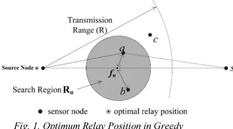
4.1. Relay Region
Relay region of any given node u is denoted as
Ru, is defined as the circle centered at u’s ideal next-hop relay position fu with radius rs(u) where rs(u) ≤
|ufu| = d0. For any node u, only the neighbors in the
relay region Ruare candidates for further forwarding
[image:3.595.317.544.329.455.2]the packets from source node u.
Fig. 1. Optimum Relay Position in Greedy Forwarding
4.2. Greedy Mode
Given any node u, let |us| be the distance from node u and sink s. Each source node calculates the
value of |us| since it knows its own position as well
as the position of sink. If the sink is in u’s
transmission range, then as per Lemma 1, direct
transmission will happen from node u to sink s.
Otherwise, the position of relay region of node u
can be computed as follows:
Let us consider (xu, yu) be the coordinate of node
u, (xs,ys) be the coordinate of sink s and (xr,yr) be the coordinate of location fu. It can be computed as follows:
When node u has a packet to forward, it
broadcasts an RTS message, which contains the
)
(
|
|
0 s u ur
us
x
x
d
x
x
=
−
−
)
(
|
|
0 s u ur
y
y
us
d
y
location of its relay region fu position as well as radius of its relay region to detect its next-hop. If a
neighbor v that gets the RTS message from node u,
it first checks if it falls in Ru. If v ≠ Ru, the RTS
message is discarded by node v. Otherwise node v
generates a CTS message which contains its calculated quality value and sets a delay, denoted by
δv→u for broadcasting the CTS message based on
delay function. When a node u receives the CTS
message from all its neighbors, it elects a single forwarder based on the quality value propagated by
hop-nodes. Finally node u unicast its packet to
next-hop relay node.
4.3. Delay Function
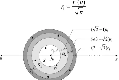
For any source node u, its search region Ru is divided into n coronas S1, S2, S3…Sn where all coronas are have same area size. Thus, the width of
ith corona is ( ) r1, where r1is the radius of S1 and
[image:4.595.88.289.388.524.2]
Fig. 2. Division of Coronas as S1, S2, S3…Sn
Therefore, given node v ɛ Ru, instead of
broadcasting CTS message instantly, node v
broadcasts its CTS message with delay δv→u. Let λ
denotes the delay for transmitting a packet from u to
v. δv→uis defined in equation 2 as follows:
(2)
4.4.Angular Relay Mode
When node u broadcasts an RTS message, it sets
its timer denoted as tmax. tmax ensures enough time to
guarantee that node u can receive CTS message
from the furthest neighbor in Ru before the timer is
expired. If node u does not receives any CTS
message before the timer is expired, then it assumes that no suitable neighbor in the search region. To recover from this local minimum, the angular relaying proposed in [13] is employed. This angular
relaying algorithm works in two phases: selection phase and protest phase. In the selection phase, the
node u broadcast RTS message to all its neighbors
without any delay function and all the neighbors answer with CTS messages in counterclockwise order according to an angular based delay function. If anyone of forwarder answers with valid CTS, the protest phase begins. First, only the nodes deployed in Gabriel circle are allowed to protest. If node v
protests, it automatically becomes the next-hop
relay to source u. After that, only nodes in NGG(u,v)
are allowed to protest. Finally node u forwards to
the elected node v.
4.5.Calculation of Quality Value
The key aspect of our work is the calculation of quality value of individual nodes. The quality value is depends on the nodes individual battery power
and its distance from optimum relay position fu.
When a node v receives an RTS message, it sets its
own delay i.e. δv→u and computes its own quality
value. The delay function specified in equation 2 ensures the required delay to each nodes to broadcasts its CTS message. Let β denotes the distance between the next-hop node coordinates (xf,yf) and optimum relay position fu = (xr,yr). As per Pythagorean Theorem,
(3)
The quality value of each node denoted as η can be derived as follows:
(4)
n
u
r
r
c(
)
1
=
1
−
−
i
i
(
)
−
−
+
−
−
=
∑
= →(
)
1
|
|
.
1
2
.
)
(
.
1
n
r
u
m
vf
m
i
n
u
r
s v m i s u vλ
λ
δ
1
)
(
|
.
2+
=
u
r
vf
n
m
s v 22
(
)
)
(
x
r−
x
f+
y
r−
y
fwhere Resiis the battery power of node i. Each node computes their quality value based on equation 3 and 4, and sends the quality value to source node along with CTS message. Whenever a source node
u receives these CTS messages, it records the
quality value along with the respective replier ID’s.
After the timer period expires, i.e. tmaxsource selects
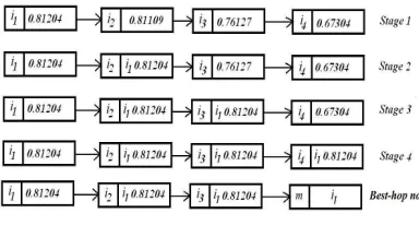
[image:5.595.95.287.243.346.2]the best-hop, which should have a maximum quality value.
Fig. 3. Selection of Best-Hop Node Based on Quality Value.
After tmax, if some recorded values are found in a
source node u, its states that few qualified forwarder
nodes are available in source node u’s optimum
relay region. Then source node u immediately
initiates the election period. At the time of election, each nodes quality value is compared with the other nodes quality values. The node which is having a greater quality value is elected by the source and the packets are unicasted to the best-hop node. The quality value computed in (3) and (4) guarantees:
1. Each node is having different quality values
based on their different coordinate locations.
2. Congestion is a due in our work, because
CTS messages are generated by δ. This
method eliminates the collisions of CTS
messages by source node u.
5. THEORETICAL ANALYSIS AND
RESULTS
In this section, we present some theoretical analysis and also simulation results for our work based on simplified MAC without considering packet loss, the UDG model without greedy failures and uniform node deployment.
5.1.Guaranteed Delivery
Let u be a source node and s be the sink. If sink s
is located in the transmission range of node u and then,
.
Here direct transmission is possible and no need of any relay nodes here.
If the case is reversed then,
then the packets may need some relay nodes before arriving sink.
5.2.Extension to Lossy Wireless Sensor Networks
Packets may be lost due to many reasons such as collision, data error or the attenuation of signal strength in the receiver. To analyze the behavior of data loss, packet reception rate (PRR) is used to measure the quality of unreliable communication
links. Let PRR(u,v)be the packet reception rate for
the communication link from u → v. The expected
rate of success in packet transmission is [PRR(u.v)]
-1
. If a packet is lost before reaching the receiver antenna, nearly same amount of energy dissipated by the listener. Therefore, the relay process of 1 bit
data from u → v can be modeled as,
E[Єtotal(u → v)] ≈
5.3.Simulation Settings
Our work is inspired by the study of RF communication rule, whose energy consumption is very large amid other functional domains. In this perspective, we have implemented a simulation package based on NS-2 [24]. In all the simulations, 500 sensor nodes are randomly deployed in 5000m x 1500m region. The sink is placed at the center of the region. Three different scenarios are designed to evaluate the performance of the proposed work. The data transmission rate of nodes is in the range
(
)
k
k
x
x
us
−
−
≤
12 1
2
1
|
|
(
)
k
k
x
x
us
−
−
>
12 1
2
1
|
|
)
,
(
|)
(|
v
u
PRR
of 250 kbps and disseminated in ISM band. The transmission range for an individual node is 25m. The sink node is understood to have an infinite power supply. Single source node can generate one packet per second. Packet size is 80 bytes, and the overall simulation setup time is 3000 seconds. We use first order radio model to compute the energy consumption. The parameter values used in the simulations are presented in Table 1. The basic settings are common to all the experiments.
Table1. Simulation settings.
Network Area 5000m x 1500m
Total Sensor Nodes 500
Data Rate at MAC layer 250 kbps
Topology Configuration Randomized
Packet loss rate 0%
Node failure rate 0%
Transmission Range 25m
Overall Simulation Time
50 minutes
• Mobility scenario: Every sensor nodes move according to Random Walk Mobility Model [25]. A sensor can select its own new location by choosing its speed and direction from the range [0,2π]. Every node is specified with interval of 10 seconds. New speed and direction can be taken at the end of each interval.
• Random Sleep Wake up Scenario: A Random Independent Sleeping (RIS) scheme proposed in [34] is employed in our work to extend the network lifetime. This RIS scheme divides the entire simulation in ζsleep. Each node decides its slot based on a probability value ρ. Node sleep schedule is given by 1 – ρ and wake up cycle is decided by ρ.
For performance analysis, in addition to GRRR, we have implemented another two schemes: BLR [11] and GPER [18]. BLR also uses geographic information and it considers hop-count routing metric. Like GRRR, BLR also follows beaconless mode to identify the next-hop in its relay region. In each simulation 25 nodes are selected as sources and each source can produce 40 data packets. Payload size is 128 bytes.
5.4.Performance of GRRR in Mobility Scenarios
In this simulation, we evaluate the
performance of GRRR in mobility scenarios in which topology changes continuously due to node mobility. The parameters of Random Walk
Mobility model are set as follows: minspeed is 0
m/s and maxspeed is varied from 0 m/s to 50 m/s to
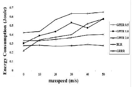
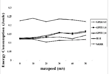
deliver different mobility levels. The simulated beacon intervals for GPER are 0.5, 1.0 and 2.0 seconds (GPER 0.5, GPER 1.0 and GPER 2.0).
Fig. 4. (a) shows the energy consumption is referred to as the sum of the energy spent by each node in the network. Here GRRR and BLR are much robust because they decide their forwarding decision based on the actual network topology. When the maxspeed increases, the energy consumption of GRRR and BLR increases slightly due to the suboptimal energy routes and slight packet drops caused by node mobility.
Fig. 4. (a) Energy Consumption
Fig. 4. (b), we observe that, when the nodes are in immovable state, the packet loss rate of BLR and GRRR almost closes to zero. On the other hand, when the nodes in mobility state, the packet drop ratio is larger in BLR and then that in GRRR because BLR tends to identify the next-hop node from its transmission range, and it is possible that the established connection may lost before receiving the packet. Node movement makes significant impact on the performance of GPER.
When the node speed is less than 5 m/s, GPER with
beacon 2.0 seconds consumes less energy than GRRR because of low packet loss and low
handshaking mechanisms. But when maxspeed
increases i.e. 50 m/s GPER with a beacon interval
[image:6.595.305.517.388.528.2]The reason behind is, the collected information is outdated quickly in GPER when the node moves in a high speed.
Fig. 4. (b),Masspeed versus Packet Drop Ratio
Fig. 4. (c) Sum of Energy Consumption along Routing Path
Fig. 4. (c) shows the sum of energy spent on the successful packet transmission. It can be seen that BLR consumes more than 80 % energy than GRRR, means that route making in BLR is not so effective. Second, BLR covers the entire forwarder nodes by broadcasting RTS messages. In contrast, GRRR broadcasts RTS message to all forwarders but eventually it approaches only the nodes which comes closer to relay region.
Fig. 4. (d) shows that the total number of control messages broadcasted in BLR is around 50 percent less that in GRRR since the total count of control messages is proportional to the number of hop-nodes. However, it doesn’t mean that the total energy spend by broadcasting control messages in BLR must be smaller than GRRR because each node spends more energy to broadcast control messages in BLR.
Fig. 4. (d) Control Message Overhead
5.5.Performance of GRRR In Random Sleep Wake Up Scenarios
In order to measure the performance of simulated protocols in random sleep wake up cycle, RIS scheme (Tshift) is integrated. For GPER, every node broadcasts a beacon message only when it
shifts between sleep and active state. For GRRR
and BLR, each node broadcasts RTS message only when it works in active state. Neighbor node will be active in the selection process if its remaining active time is large enough to complete forwarding one data packet.
[image:7.595.305.517.159.301.2] [image:7.595.83.288.171.315.2] [image:7.595.83.292.349.491.2]Fig. 5. (a) Energy versus Sleeping Probability
Fig. 5. (b) Energy versus Time Interval in RIS
Fig. 5. (b) shows the energy consumption of all
the three protocols when the time interval (Tshift) is
changing. Here node sleeping probability value is
set as 50% and packet generation ratios are 1
packet/5 sec and 1 packet/10 sec. It is observed that
GRRR and BLR is independent to Tshift because
their selection process depends on the number of active nodes in their region. It’s also observed that the required control messages for GRRR and BLR is also significantly reduced. GPER forwards the packet based on collected information. When the interval time is high, collected neighborhood information will be quickly outdated. As shown in Fig. 5. (b), GPER outperforms than GRRR and
BLR when Tshift increases. Because GPER losses
very low energy since it exchanges minimum beacon messages. It is worth to notice that GPER with low data generation consumes more energy than GPER with high data transmission rate because the forwarding time with low data generation is long and more beacon messages are
required for communication. Thus, in contrast to GPER, GRRR is most suitable for event-detection applications in which data generation rate is low.
6. CONCLUSION
Power aware routing is an important issue in WSNs. In this work, we propose a novel power aware geographic routing GRRR which takes the advantage of both geographic routing and power aware routing to provide energy efficient, loop-free,
stateless sensor-to-sink routing in dynamic
scenarios. The performance of GRRR is evaluated under different cases. Simulation results show that our protocol outperforms well in most scenarios and also consumes less power than other protocols based on neighborhood information in highly dynamic scenarios.
REFERENCES
[1] Akyildiz, I. F., Su, W., Sankarasubramaian, Y., & Cayirci, E. (2002). A Survey on Sensor
Networks. IEEE Communication Magazine,
Vol. 40, Issue. 8, 102 – 114.
[2] Al-Karaki. J., & Kamal. A. (2004). Routing techniques in Wireless Sensor Networks: a
survey, IEEE Transactions on Wireless
Communications, Vol.11, Issue 6, 6 – 28. [3] Akkaya. K., & Younis. M. F. (2005). A
Survey on Routing Protocols for Wireless
Sensor Networks, IEEE Transactions on
Ad-hoc Networks, Vol. 3, Issue.3, 325 – 349. [4] Hsin. C., & Liu. M. (2004). Network
Coverage Using Low Duty-Cycled Sensors: Random and Coordinated Sleep Algorithms,
Proceedings of Third International Symposium in Information Processing in Sensor Networks, 433-442.
[5] Kumar. S., Lai. T. H., & Balogh. J. (2004). On K-coverage in a Mostly Sleeping Sensor
Network, Proceedings of ACM MobiCom,
144-158.
[6] Frey. H., & Stojmenovic. I. (2006). On Delivery Guarantees of Face and Combined Greedy-Face Routing in Ad Hoc and Sensor
Networks, Proceedings of ACM MobiCom,
390-401.
[7] Blum. B, He. T., Son. S., & Stankovic. J.
(2003). IGF: A State-Free Robust
Communication Protocol for Wireless Sensor
Networks, Technical Report CS-2003-11,
[image:8.595.88.287.319.472.2][8] Fußler. H., Widmer. J., Kasemann. M., Mauve. M., & Hartenstein. H. (2003). Contention-Based Forwarding for Mobile Ad
Hoc Networks, Ad Hoc Networks, vol. 1,
351-369.
[9] Zhang. H., & Shen. H. (2007). EEGR: Energy-Efficient Geographic Routing in
Wireless Sensor Networks,” Proceedings of
IEEE International Conference on Parallel Processing.
[10] Chawla. M., Goel. N., Kalaichelvan. K., Nayak. A., & Stojmenovic. I. (2006). Beaconless Position Based Routing with Guaranteed Delivery for Wireless Ad-Hoc
and Sensor Networks, Proceedings of FIP
International Federation for Information Processing World Computer Congress, 61-70. [11] Heissenbuttel. M., Braun. T., Bernoulli. T., & Walchli. M. (2004). BLR: Beacon-Less Routing Algorithm for Mobile Ad Hoc
Networks, Computer Communications, vol.
11, 1076-1086.
[12] Zhang. H., & Shen. H. (2010). EBGR:
Energy-Efficient Beaconless Geographic
Routing in Wireless Sensor Networks,” IEEE
Transactions on Parallel and Distributed Systems, Vol. 21, 881-896.
[13] Barriere. L., Fraigniaud. P., Narayanan. L., & Opatrny. J. (2003). Robust Position-Based Routing in Wireless Ad Hoc Networks with
Irregular Transmission Ranges, Wireless
Communications and Mobile Computing, vol. 3, 141-153.
[14] Singh. S., Woo. M., & Mghavendra. C. S. (1998). Power-Aware Routing in Mobile Ad
Hoc Networks, Proceedings of ACM
MobiCom, 181-190.
[15] Stojmenovic. I & Lin. X. (2001). Power-Aware Localized Routing in Wireless
Networks, IEEE Transactions on Parallel and
Distributed Systems, vol. 12, no. 11, 1122-1133.
[16] Kalpakis. K., Dasgupta. K., & Namjoshi. P. (2003). Efficient Algorithms for Maximum Lifetime Data Gathering and Aggregation in
Wireless Sensor Networks, Computer
Networks, vol. 42, pp. 697-716.
[17] Takagi. H., & Kleinrock. L. (1984). Optimal
Transmission Ranges for Randomly
Distributed Packet Radio Terminals, IEEE
Transactions on Communications, vol. COM-32, no. 3, 246- 257.
[18] Wu. S., & Candan. K. S. (2004). GPER: Geographic Power Efficient Routing in
Sensor Networks,” Proceedings of IEEE
International Conference in Network Protocols 161-172.
[19] Kuruvila. J., Nayak. A., & Stojmenovic. I. (2004). Hop Count Optimal Position Based Packet Routing Algorithms for Ad Hoc Wireless Networks with a Realistic Physical
Layer,” Proceedings of First IEEE
International Conference on Mobile Ad-Hoc and Sensor Systems, 398-405.
[20] Bose. I. S. P., Morin. P., & Urrutia. J. (1999). Routing with Guaranteed Delivery in Ad Hoc
Wireless Networks, Proceedings of Third
ACM International Workshop Discrete Algorithms and Methods for Mobile Computing and Communications, 48-55. [21] Karp. H. T. K. B. (2000). GPSR: Greedy
Perimeter Stateless Routing for Wireless
Networks, Proceedings of ACM MobiCom,
243-254.
[22] Kuhn. F., Wattenhofer. R., & Zollinger. A. (2003). Worst-Case Optimal and Average-Case Efficient Geometric Ad-Hoc Routing,
Proceedings of ACM MobiCom, 267-278, 2003.
[23] Heinzelman. W. R., Chandrakasan. A., & Balakrishnan. H. (2000). Energy-Efficient
Communication Protocol for Wireless
Microsensor Networks, Proceedings of 33rd
Hawaii International Conference on System Sciences, 4-7.
[24] http://www.isi.edu/nsnam/ns/
[25] Sanchez. M., & Manzoni. P. (1999). A
Java-Based Ad Hoc Networks Simulator,