ANALYSIS OF TRAFFIC FLOW IN CONGESTED CITIES
USING CELLULAR AUTOMATA
1S.RAJESWARAN AND 2S.RAJASEKARAN
1 Department of Mathematics, Velammal Engineering College, Chennai-66 2
Department of Mathematics, B.S.Abdur Rahman University, Chennai-48 Email: [email protected], [email protected]
ABSTRACT
The present study is to model heterogeneous traffic at a congested place in Chennai using Cellular Automata (CA) and traffic simulator VISSIM. Vehicle type, its volume, density, average velocity, dimensions of study area and signal cycle length are used as input parameters for computer simulator VISSIM to find the dynamics of vehicular traffic. The output obtained substantiates that there will be decrease in delay time and increase in maximum achievable velocity when there is reduction in 2W (Two Wheeler) population. In fact, if no 2W is allowed then the delay time will be reduced to 70.70% and the maximum achievable velocity will be increased to 34.33%. Using CA rules, simulation was carried out on the traffic flows in roads of length 100 (small system) and 1000(large system). The results obtained show that small systems behave differently from long ones and the traffic reaches a maximum of 420 when the density is 0.1 for small systems and 323 when the density is 0.09 for large system.
Keywords: Cellular Automata, Heterogeneous Traffic, Vehicular Traffic, Single-Lane Traffic Flow, Simulation.
1. INTRODUCTION
In a developing country like India vehicular traffic is a major problem since the growth of traffic is exponential and traffic conditions are heterogeneous. Chennai is one of the cities with heavy traffic congestion and a chaotic transport system. This is due to the roaming of more than 7 million inhabitants, 55000 taxis, 18000 buses and 1 million private cars in the city streets. In spite of introducing mass transportation system, erecting pedestrian bridges, making one-ways and restricting the movement of heavy vehicles in peak hours the management could not solve this problem. Unless the dynamics of vehicular traffic and the behavior of drivers are known it is impossible to solve this problem. To study effectively the dynamics of vehicular traffic, Mathematical modeling and computer simulation techniques can be used. In this present study microscopic models such as Cellular Automata (CA) and traffic simulator VISSIM are used to study the dynamics of vehicular traffic and the behavior of drivers.
1.1 Objectives of the Study
The main aim of the present study is modeling of traffic flow at a congested place in Chennai, using
CA and traffic simulator VISSIM. Based on the congested report of the traffic department of Chennai city, Spencer intersection is chosen as our study area. Using various primary traffic surveys, vehicle type, its volume, density, average velocity, dimensions of study area, signal cycle length etc are identified and are used as input parameters for computer simulator VISSIM to find the dynamics of vehicular traffic. Basic rules for the CA model are discussed from these dynamics of vehicular traffic. Three different traffic flow conditions viz traffic condition with 25% less two wheeler (2W) traffic, 50% less 2W traffic and 100% less 2W traffic are studied using VISSIM. The output obtained by using the computer simulation software VISSIM is easily interpretable. Very useful basic CA rules are presented for future microscopic modeling of heterogeneous traffic in Chennai city.
1.2 Description
and model is created. This model provides the traffic condition and the dynamic properties of the vehicles. With suitable assumptions the future traffic is predicted. Conclusion is drawn after studying the traffic conditions with 25% less 2W traffic, 50% less 2W traffic and 100% less 2W traffic. For the future microscopic modeling of traffic flow in the congested cities the basic concept of CA are presented in this paper.
2. LITERATURE REVIEW
Mainly there are 2 approaches available in modeling of traffic flow. The first approach (Car-following model) treats the individual cars and the second approach describes the dynamics of traffic networks in terms of macroscopic variables. The assumption made in the first approach is that the behavior of a driver is determined by the leading vehicle. This assumption leads to dynamical equations which are depending on the distance of the leading vehicles and also the difference between velocities of the leading vehicle and the one following it. In the first approach we encounter difficulty to treat in computer simulations. Even though the large networks can be treated in principle the macroscopic approaches lead to some difficulties and the information obtained cannot trace back individual cars. To avoid these difficulties CA models which are microscopic in nature are designed. However, in general the CA models for urban traffic do not address the issues arise out of heavy traffic in crowded cities.
The concept of CA was first used by Nagel and Schreckenberg [1] to develop traffic flow models. This concept has got several computational advantages in modeling complex systems. Some modifications were made by Takaryasu [2], Schadschneider and Schreckenberg [3], and Barlovic et al [4] to address the important features observed in real traffic situations and were aimed at modeling the outflow from jam and velocity of the upstream front of the jam. In discrete optimal velocity model vehicle acceleration and deceleration behavior is modified. Knospe et al [5] proposed brake light model. In this model car following behavior is independent on brake light status of the leading and following vehicles. The above mentioned models are all single lane models which do not address the reality. Hence, two lane CA models are developed by Rickert et al [6], Chowdhury et al [7], Wagner et al [8], Nagel et al [9] and Knospe et at [10]. Among the models, the one due to Knospe is more successful in modeling microscopic behavior of the traffic.
Recently, Lan and Chang [11] using refined CA structure modeled mixed traffic composed of cars and 2 wheelers. However it has failed to model several observed traffic features. Again using refined CA structure Lan and Hsu [12] attempted to model the effect of moving bottleneck on the homogeneous traffic stream. Even these models have failed to model several observed mixed traffic features. However, CA models have been applied with success to traffic simulations and are able to reproduce the macroscopic behavior of each car. Some theoretical and practical studies were made to extend these models to two and three-lane highways.
3. THE STUDY AREA
3.1 Definition of the Study Area
The study area can be at the national level, the region level or urban level. We restrict ourselves at the urban level. The study area in urban level is a metropolitan area. The boundary of the study area is termed as “external cordon”. Detailed surveys are conducted and the economic activities are studied intensively inside the study area to determine the travel characteristics.
3.2 Selection of Study Area
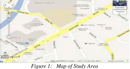
[image:2.612.313.524.551.663.2]The Spenser intersection on the Anna Salai, Chennai has been chosen as our study area for traffic modeling since this is one of the congested intersections on the congested road Anna Salai having the properties that the roads leading to this intersection have no curves so that it is easy for traffic modeling and the dimensions of these roads are good enough to study dynamic properties. The map of the study area is shown in Fig 1. The data required for the traffic modeling are of two types viz Primary Data and Secondary Data.
Figure 1: Map of Study Area
3.3 Survey for the Primary Data
(i) Volume count (ii) Types of vehicles (iii) Turning moment (iv) Road geometry.
For the primary data collection, the study area is divided into four zones pertaining to four roads forming the intersection. The types of vehicles on the road are grouped as Two Wheeler (2W), Car (4W), Bus (B), and Heavy Vehicle (HV). For each zone, each type of vehicle two persons are required for counting its volume. These volume data are recorded. From which peak volume and peak hours can be easily found out.
4. TRAFFIC VOLUME DETAILS OF ANNA SALAI
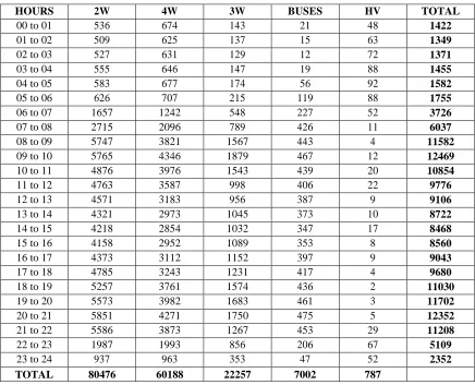
[image:3.612.93.291.310.441.2]The hourly traffic volume of Anna Salai is shown in table 1. Based on this data Fig 2 gives the Vehicle distribution chart of Anna salai.
Figure 2: Vehicle Distribution Chart of Anna Salai
4.1 Spenser Intersection Traffic Volume Details
The Spenser intersection has six possible routes. Six routes are divided into six zones. The traffic volume of each zone per hour is tabulated below.
4.2 Secondary Data
Secondary data corresponds to vehicle properties and road dimensions. The following are classified as secondary data.
1. Vehicle dimensions 2. Average velocity
3. Average time taken to clear the signal 4. Gap between two vehicles in a signal 5. Brake gap
6. Acceleration gap 7. Signal cycle length
4.3 Survey for Secondary Data
Vehicle dimensions are got by measuring with survey tape and through vehicle prospectus. Average velocity, average time required to clear the signal are calculated by sitting in a car and traveling the trip distance. Gap between two vehicles in a signal, brake gap and acceleration gap are obtained by suitable assumptions from the video clips of the intersection.
Transportation today plays an important role in the economic and physical development of any modern city. Today, many micro-simulation software have been made available on the market and used as tools for the evaluation of traffic management and control. Released in 1992, VISSIM is a microscopic, time step and behavior based simulation model developed by PTV, Planung Transport Verkehr AG in Karlsruhe,Germany to model urban traffic and public transit operations. VISSIM is the abbreviation of "Verkehr In Städten SIMulationsmodell". It is regarded today as a leader in the arena of micro-simulation software.
4.3.1 Methodology
All the vehicles on road are classified according to their types. Since VISSIM does not have 3W input, all the 3W are converted in terms of 4W by equivalence factor. Each type of vehicles i s again classified according to their velocity. All the parameters those were required as inputs are taken from primary and secondary data. The traffic model was simulated from 00 seconds to 600 seconds. The traffic condition with reduction in two wheeler population is studied.
4.3.2 Input
This model requires study area map, which represents actual study area; lane linking, which shows the direction of traffic; signal position, which represents the stop line; signal cycle length; vehicle types and their average velocity; distribution of traffic, which represent the traffic in each zone; simulation time, which represents the time for which the traffic is to be simulated.
4.3.3 Input pictures
Figure 3: Digitalized Image of Study Area
5. OUTPUT
On simulating the model we can get our desired output such as delay time, maximum desired velocity and maximum achievable velocity. These parameters are studied for different rates of 2W population reduction.
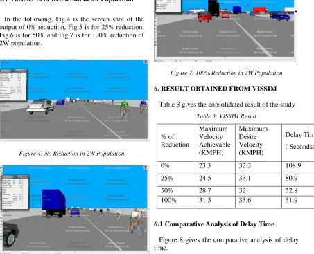
5.1 Various % of Reduction in 2w Population
In the following, Fig.4 is the screen shot of the output of 0% reduction, Fig.5 is for 25% reduction, Fig.6 is for 50% and Fig.7 is for 100% reduction of 2W population.
Figure 4: No Reduction in 2W Population
Figure 5: 25% Reduction in 2W Population
[image:4.612.316.521.249.398.2]
Figure 6: 50% Reduction in 2W Population
Figure 7: 100% Reduction in 2W Population
[image:4.612.91.544.303.670.2]6. RESULT OBTAINED FROM VISSIM
Table 3 gives the consolidated result of the study
Table 3: VISSIM Result
% of Reduction
Maximum Velocity Achievable (KMPH)
Maximum Desire Velocity (KMPH)
Delay Time ( Seconds)
0% 23.3 32.3 108.9 25% 24.5 33.1 80.9 50% 28.7 32 52.8 100% 31.3 33.6 31.9
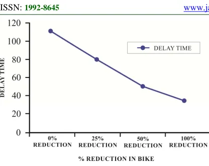
6.1 Comparative Analysis of Delay Time
Figure 8: Comparative Analysis of Delay Time
6.2 Comparative Analysis of Maximum Velocity Achievable
Figure 9 shows the comparative analysis of maximum velocity achievable.
Figure 9: Comparative Analysis of Maximum Achievable Velocity
7. CA TRAFFIC FLOW MODELS
This model is a microscopic traffic model. In this model time is made into discrete variable and the roadway is divided into cells so that vehicles move from one cell to another. Nagel and Scheckenberg [1] were the first to use CA models for traffic simulation. They have used a stochastic CA model to simulate a single-lane highway traffic flow. In the traffic flow, the basic rule is the movement of each vehicle to
v
sites at each time. There are some CA models that have been used as frequently as the models due to Nagel-Schreckenberg [1] and BJH model [13]. In the CA model, the street is divided into cells, each of length depending on the length of the car and the distance to the precedingcar. Each cell is occupied by at most one car and the velocity of each car is between 0 and
v
max.The simplest traffic CA model is one developed by Wolfram [14] and Biham et. al.[15]. In this model the formula connecting the positions of the ith vehicle at time t and t+1 is given by
)
,
1
(
min
)
(
)
1
(
i ii
t
x
t
d
x
+
=
+
(1)where
d
i=
x
i+1(
t
)
−
x
i(
t
)
−
1
Fukui and Ishibashi extended this model by modifying the above relation as
)
,
(
min
)
(
)
1
(
i max ii
t
x
t
v
d
x
+
=
+
, (2)by assuming the existence of the maximum speed
v
max.7.1 Simplest Rule Set of Nagel-Schreckenberg (Nasch) Model
The following is a set of rules introduced by Nagel and Schreckenberg .
Rule1. All the vehicles whose velocity has not reached the maximum velocity
v
maxwill accelerate by one unit.(i.e)
v
i→
v
i'=
v
i+
1
,
if
v
i<
v
max (3)Rule2. Let
d
ibe the distance along the road, separating car i and i+1. If the velocity of the car(v
)
is greater thand
i, then the velocity becomesd
i. If the velocity of the car(v
)
is smaller thand
i , then the velocity becomesv
.(i.e)
v
i'→
v
i"=
d
i−
1
,
if
v
i'≥
d
i (4)Rule3. The velocity of the car may reduce by one unit with the probability
p
i.(i.e)
v
i'
'
→
v
i'
''
=
v
i'
'
−
1
,
with probabilityi
p
if v
i''
>
0
(5)Rule4. After 3 steps, the new position of the vehicle can be determined by the current velocity and current position.
[image:5.612.88.300.322.493.2]7.2 Algorithm for Single-Lane Traffic Model
Input
The length of the highway, The length of the cell, Maximum velocity, Initial density, Incident details and Driver behavior probability p.
Initialization
Generate Initial vehicles. Begin
Calculate gap
g
i=
x
i−
x
i−1Acceleration
v
i→
min
(
v
i+
1
,
v
max)
Deceleration
v
i→
min
(
v
i,
g
i−
1
)
Randomization
v
i→
max
(
v
i−
1
,
0
)
withprobability p
Vehicle position update
x
i→
x
i+
v
i [image:6.612.81.525.67.370.2]Vehicle generation
Figure 10: Algorithm for Single-Lane Traffic
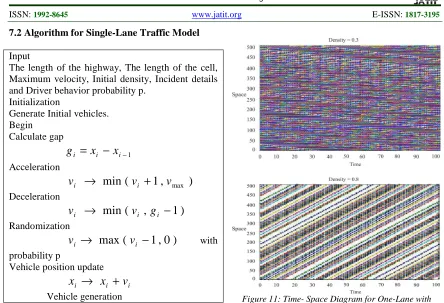
7.3 Simulation of Single-Lane Traffic Flow
In order to simulate single-lane traffic flow, first we define there are 500 cells in the roadway and then we randomly generate the position and speed for each car. Further, we assume that the probability of a car driver to slow down the speed is, given by p = 0. Time-space diagrams are used to show the movements of vehicles. We choose the last 100 movements of 500 step movement. CA model can avoid the noise in the absence of slow down step.
[image:6.612.216.537.568.714.2]
Figure 11: Time- Space Diagram for One-Lane with Density = 0.1, 0.3, and 0.8.
7.4 Experiment for A Single Lane
Using the CA rules mentioned in Section 7.1, simulation was carried out to see the difference in the traffic flows between road length L = 100 ( small system) and L = 1000( large system):
The density (ρ) is the number of cells in which a
car exists divided by the total number of cells and traffic (q) is the number of cars that pass a certain cell with in a fixed time. The following figure shows the relation between density and traffic in case of small system as well as large system, by considering the 50th cell and the fixed time limit t = 0 to t = 1000 to get q :
The above figure shows that for small systems the model reaches the maximum capacity q = 420 at a density of ρ = 0.1 whereas for large systems q =
323 at a density of ρ = 0.09. That is short segments
behave differently from long one. Figure also reveals that due to congestion the traffic decreases at ρ = 0.09.
8. CONCLUSION
Three traffic flow conditions namely traffic condition with 25% less 2W traffic, 50% less 2W traffic and 100% less 2W traffic were considered. There is a substantial decrease in delay time with reduction in 2W population. If no 2W is allowed in the Anna Salai, then delay time can be reduced to 70.70%. Maximum achievable velocity can be increased to 34.33% if no 2W is allowed on Anna Salai. Using CA rules, simulation was carried out on the traffic flows in roads of length 100 (small system) and 1000 (large system). The results obtained show that small systems behave differently from long ones and the traffic reaches a maximum of 420 when the density is 0.1 for the small system and 323 when the density is 0.09 for the large system. Very useful CA rules are presented for future microscopic modeling of heterogeneous traffics in congested cities.
REFERENCES:
[1]Nagel, K. and Schreckenberg, M., “A cellular automaton model for freeway traffic”, Journal of Physics I France 2, 2221-2229, 1992.
[2]Takayasu, M. and Takayasu, H., “1/f noise in a traffic model”, Fractals 1(4), 860-866, 1933. [3]Schadschneider, A. and Schreckenberg, M.,
“Traffic flow models with ‘slow-to-start’ rules”, Ann. Physik 6, 541-551, 1997.
[4]Barlovic, R., Santen, L., Sahadschneider, A., and Schreckenberg, M., “Metastable states in cellular automata for traffic flow,” Eur.Phys.Journal B5, 793-800, 1998.
[5]Knospe, W., Santen, L., Schadschneider, A., and Schreckenberg, M., “Empirical test for cellular automaton models of traffic flow”, Physical Review E (Statistical, Nonlinear, and Soft Matter Physics), 70(1), 016115-016125, 2004.
[6]Rickert, M., Nagel, K., Schreckenberg, M., and Latour, A., “Two lane traffic simulation using cellular automata”, Physica A: Statistical and Theorectical Physics 231(4), 534-550, 1996.
[7]Chowdhury, D., Wolf, D.E., and Schreckenberg, M., “Particle hopping models for two-lane traffic with two kinds of vehicles: Effects of lane-changing rules”, Physica A: Statistical and Theorectical Physics 235(3-4), 417-439, 1997. [8]Wagner, P., Nagel, K., and Wolf, D. E., “Realistic
multi-lane traffic rules for cellular automata”, Physica A: Statistical and Theoretical Physics 235(3-4), 687-698, 1997.
[9]Nagel, K., Wolf, D. E., Wagner, P., and Simon, P., “Two lane traffic simulations using cellular automata: A systematic approach”, Physical Review E 58920, 1425-1437.
[10]Knospe, W., Santen, L., Schadschneider, A., and Schreckenberg, M., “Towards a realistic microscopic description of highway traffic”, Journal of Physics A, Mathematical and General (48), L477-L485, 2000.
[11]Lan, W. L., and Chang, C. W., “Inhomogeneous Cellular Automata modeling for mixed traffic with cars and motorcycles”, Journal of Advanced Transportation 39, 323-349, 2005. [12]Lan, W. L., and Hsu, C., “Formation of
Spatiotemporal Traffic patterns with Cellular Automaton Simulation”, TRB 2006 Annual Meeting CD-ROM, 2006.
[13]Benjamin, S. C., Johnson, N. F., Hui, P. M., “Cellular automata models of traffic flow along a highway containing a junction”, Journal of Physics A: Mathematical and General 29 (12) 3119-3127, 1996.
[14]Wolfram, S., “Theory and applications of Cellular Automata”, Singapore: World Scientific, 1986.
Table 1: Hourly Traffic Volume of Anna Salai
Table 2: Volume of Six Zones Per Hour
S.No. Vehicle
Type
Gemini to Central
Zone
Gemini to Ethiraj
Zone
Ethiraj to Gemini
Zone
Central to Gemini
Zone
Ethiraj to Central
Zone
Central to Ethiraj
Zone
1. 2Ws 3072 1521 833 2834 795 771 2. Cars 2256 773 761 2190 621 717 3. Autos 636 453 261 694 194 218 4. Buses 216 104 34 217 0 0 5. HVs 102 97 38 81 34 20
HOURS 2W 4W 3W BUSES HV TOTAL
00 to 01 536 674 143 21 48 1422
01 to 02 509 625 137 15 63 1349
02 to 03 527 631 129 12 72 1371
03 to 04 555 646 147 19 88 1455
04 to 05 583 677 174 56 92 1582
05 to 06 626 707 215 119 88 1755
06 to 07 1657 1242 548 227 52 3726
07 to 08 2715 2096 789 426 11 6037
08 to 09 5747 3821 1567 443 4 11582
09 to 10 5765 4346 1879 467 12 12469
10 to 11 4876 3976 1543 439 20 10854
11 to 12 4763 3587 998 406 22 9776
12 to 13 4571 3183 956 387 9 9106
13 to 14 4321 2973 1045 373 10 8722
14 to 15 4218 2854 1032 347 17 8468
15 to 16 4158 2952 1089 353 8 8560
16 to 17 4373 3112 1152 397 9 9043
17 to 18 4785 3243 1231 417 4 9680
18 to 19 5257 3761 1574 436 2 11030
19 to 20 5573 3982 1683 461 3 11702
20 to 21 5851 4271 1750 475 5 12352
21 to 22 5586 3873 1267 453 29 11208
22 to 23 1987 1993 856 206 67 5109
23 to 24 937 963 353 47 52 2352