http://dx.doi.org/10.4236/jqis.2016.61006
The Pancharatnam Phase of a Three-Level
Atom Coupled to Two Systems of N-Two
Level Atoms
D. A. M. Abo-Kahla
Department of Mathematics, Faculty of Education, Ain Shams University, Cairo, Egypt
Received 7 February 2016; accepted 25 March 2016; published 30 March 2016
Copyright © 2016 by authors and Scientific Research Publishing Inc.
This work is licensed under the Creative Commons Attribution International License (CC BY). http://creativecommons.org/licenses/by/4.0/
Abstract
In this paper, we present the analytical solution for the model that describes the interaction be-tween a three-level atom and two systems of N-two level atoms. The effects of the quantum num-bers and the coupling parameters between spins on the Pancharatnam phase and the atomic in-version, for some special cases of the initial states, are investigated. The comparison between the two effects shows that the analytic results are well consistent.
Keywords
Pancharatnam Phase, Atomic Inversion, Systems of N-Two Level Atoms
1. Introduction
The use of statistical mechanics is fundamental to the concepts of quantum optics: Light is described in terms of field operators for creation and annihilation of photons [1]-[7]. Features of quantum optics are mainly based on three different types of interaction, namely, field-field, atom-atom, atom-field interaction. Each one of these in-teractions represents a certain type of physical phenomena [8]-[13]. For example, Hichem Eleuch and Raouf Bennaceur studied the interaction between a three-level system in the lambda configuration with two resonant electromagnetic fields, through which the motion of a pair of solitons propagating through an absorbing three- level system in the lambda configuration was analyzed [14].
In addition, based on Dicke’s superradiance, Eyob A. Sete et al. studied the collective spontaneous emission from an ensemble of N identical two-level atoms prepared by absorption of a single photon—a.k.a. single pho-ton Dicke superradiance [15].
inte-raction between a three-level atom and two systems of N-two level atoms. The time evolution of dynamical sys-tems has attracted considerable attention over the past several decades because of its various applications. An important aspect in this regard is the quantum phase associated with the evolution of these states in certain cir-cumstances [16].
In recent years much attention has paid to the quantum phases [17] such as the Pancharatnam phase [18]-[22] and the geometric phase [23][24]. The concept of geometric phase naturally arises for polarized light in optics. Simple quantum gates using geometric phase have been demonstrated experimentally in the nuclear magnetic resonance setup [25]. In the fifties, Pancharatnam [26] came up with a rigorous prescription for the phase ac-quired in a completely general evolution of a system. Pancharatnam discovered that when the polarization state of a beam of light was taken around a closed circuit in the state space, namely the Poincar. Sphere, it acquires an extra phase which is equal to half the solid angle subtended by the circuit at the origin of the sphere [27]. In 1956, Pancharatnam [26] studied how the phase of polarized light changed after a cyclic evolution of its polari-zation [28]. In 1984 Berry addressed a quantum system undergoing a unitary and cyclic evolution under the ac-tion of a time-dependent Hamiltonian [29]. The process was supposed to be adiabatic, meaning that the time scale of the system’s evolution was much shorter than the time scale of the changing Hamiltonian [30].
The Pancharatnam phase or most commonly Berry phase is a phase difference acquired over the course of a cycle when a system is subjected to cyclic adiabatic processes, which results from the geometrical properties of the parameter space of the Hamiltonian. The Pancharatnam phase is very important in the propagation of a light beam where its polarization state is changing periodically [18]. Hence, we study the Pancharatnam phase of a three-level atom coupled to two systems of N-two level atoms as an application.
This paper is organized as follows: in section 2, we will describe the Hamiltonian of the system of interest, and obtain the explicit analytical solution of the model describing the interaction between a three-level atom and two systems of N-two level atoms. The case discussed in this paper is considered to be the generalization of the atom-atom interaction, and most of the previous papers which handled this interaction are, for the most part, considered to be a special case of our case. In section 3, different cases are studied to demonstrate the effects due to both the quantum numbers m1, m2 and the coupling parameters between spins λ1, λ2 on the atomic inver-sion Sz of the model. By analytical calculations in section 4, we examine the influence of the quantum numbers m1, m2 and the coupling parameters between spins λ1, λ2 on the Pancharatnam phase P t
( )
of the model. In section 5, we discuss the second-order correlation function where the examination of the second-order correlation function leads to better understanding for the nonclassical behavior of the system. Finally, section 6 presents the conclusions and an outlook.2. The Model
The Hamiltonian of our model describes the interaction between a three-level atom coupled to two systems of N-two level atoms. In this case the Hamiltonian of the whole system can be written in the form:
0 int.,
H=H +H (1) where,
( ) 3
2 0
1 1
,
z
H J S
β α
α
α β ββ
α β
ω =
=
= =
=
∑
+∑
Ω (2)( )1 ( )1 ( )2 ( )2 . 1 21 12 2 32 23 ,
int
H =λ S J+ +J S− +λ S J+ +J− S (3)
( )
1
1
, , , ,
2
N k
L L
k
J L x y z
α α
α
α σ
=
=
∑
= (4)1 2 3,
Ω > Ω > Ω (5)
( ) ( ) ( ),
x y
J±α =Jα ±iJα (6)
[
Skl,Snm]
=Skmδnl−Snlδkm, (7)while J±( )α and Jz( )
α
are the collective angular momentum operators for N-two level atoms, which satisfy the relations
( ) ( ) ( )
, 2 z ,
J+α J−β Jαδαβ
=
(8)
( ), ( ) ( ) ,
z
Jα J±β J±αδαβ
= ±
(9)
and
( )
(
)(
)
( )
, 1 , 1 ,
, , ,
z
J j m j m j m j m
J j m m j m
α
α α α α α α α α
α
α α α α α
± = ± + ±
=
(10)
with the operator k L
α
σ is the usual Pauli matrices. We define
( )
0( )
0 ,( )
0j m s
Ψ = Ψ Ψ (11)
( )
0 j m, j m j m1, 1, 2, 2Ψ = (12)
( )
0( )
0 1( )
0 2( )
0 3s a b c
Ψ = + + (13)
( )
2( )
2( )
20 0 0 1
a +b + c = (14)
Let
( )
( )
( )
( )
1 2 1 2
1 2
, 1 1 2 2 , 1 1 2 2
, 1 1 2 2
1, , , , 2, , 1, ,
3, , 1, , 1 .
m m m m
m m
t A t j m j m B t j m j m
C t j m j m
Ψ = + +
+ + + (15)
From Schrödinger equation
( )
( )
,i t H t
t
∂ Ψ = Ψ
∂ (16)
we get from Equations (1), (15)
( )
( )
( )
( )
1 2
1 2 1 2
,
1 , 1 1 ,
d
, d
m m
m m m m
A t
i A t m B t
t =α + Λ (17)
( )
( )
( )
( )
( )
( )
1 2
1 2 1 2 1 2
,
2 , 1 1 , 2 2 ,
d
, d
m m
m m m m m m
B t
i B t m A t m C t
t =α + Λ + Λ (18)
( )
( )
( )
( )
1 2
1 2 1 2
,
3 , 2 2 ,
d
, d
m m
m m m m
C t
i C t m B t
t =α + Λ (19)
where,
(
)
1 1m1 2m2 1 ,
α = ω +ω + Ω (20)
(
)
2 1 m1 1 2m2 2,
α =ω + +ω + Ω (21)
(
)
(
)
3 1 m1 1 2 m2 1 3,
α =ω + +ω + + Ω (22)
(
)(
1)
1, 2,k
λ
k jk mk jk mk kwhere λk is the coupling parameters between spins. Define
( )
( )
1( ) ( )
2( ) ( )
31, 2 e , 1, 2 e , 1, 2 e
i t
i t i t
m m m m m m
A t =a t −α B t =b t −α C t =c t −α (24)
by substituting from Equation (24) in Equations (17)-(19) we get the following equations:
( )
1( ) ( )
21 1 d
e e ,
d
i t i t
a t
i m b t
t
α α
− = Λ −
(25)
( )
2( ) ( )
1( ) ( )
31 1 2 2
d
e e e ,
d
i t
i t i t
b t
i m a t m c t
t
α
α α −
− = Λ − + Λ
(26)
( )
3( ) ( )
22 2 d
e e ,
d
i t i t
c t
i m b t
t
α α
− = Λ −
(27)
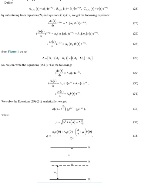
from Figure 1 we set
(
)
(
)
1 1 2 2 3 2 .
ω
ω
∆ = − Ω − Ω = Ω − Ω − (28)
So, we can write the Equations (25)-(27) as the following:
( )
( )
1 d e , d i t a ti b t
t
− ∆
= Λ (29)
( )
( )
( )
1 2
d
e e ,
d
i t i t
b t
i a t c t
t
∆ ∆
= Λ + Λ (30)
( )
( )
2 d e . d i t c ti b t
t
− ∆
= Λ (31)
We solve the Equations (29)-(31) analytically, we get:
( )
2(
)
1 2
e e e ,
i t
i t i t
b t q µ q µ
∆
−
= + (32)
where,
(
)
2 2 2
1 2
4 ,
µ = ∆ + Λ + Λ (33)
( )
( )
( )
1 2
1
0 0 0
2
, 2
a c b
q
µ
µ ∆
Λ + Λ + +
[image:4.595.82.548.95.699.2]= (34)
Figure 1. Scheme of the interaction between a three-level
( )
( )
( )
1 2
2
0 0 0
2
, 2
a c b
q
µ
µ ∆
−Λ − Λ − −
= (35)
similarly
( )
2 1 21 3
e e
e ,
2 2
i i t i t
t q q
a t q
µ µ µ µ ∆ − −
= −Λ − +
∆ ∆
− +
(36)
( )
1 23 0 1
2 2 q q q a µ µ
= + Λ ∆ − ∆
− +
(37)
and
( )
2 1 22 4
e e
e ,
2 2
i t i t i t
q q
c t q
µ µ µ µ ∆ − −
= −Λ ∆ − ∆ +
− +
(38)
( )
1 24 0 2
2 2 q q q c µ µ
= + Λ ∆ − ∆
− +
(39)
So from Equation (24) we get
( )
( )
1, 2 , 1, 2
m m m m
A t B t and
( )
1, 2 .
m m
C t
As applications to the solution of our case, a three-level atom coupled to two systems of N-two level atoms, we calculate the atomic inversion, the Pancharatnam phase and the correlation functions.
3. The Atomic Inversion
The atomic population inversion
( )
( )
( )
1 2 1 2 1 2
2 2 2
, , ,
z m m m m m m
S = A t + B t −C t , can be considered as one of the simplest important quantities, it is defined as “the difference between the probabilities of finding the atom in their exited states and in its ground state”.
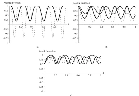
In Figures 2(a)-(c), we consider (Δ = 0, λ1 = λ2 = 1 and j1 = 30, j2 = 20). We investigate the effect of the quantum numbers m1, m2 on the atomic inversion. In Figure 2(a), the initial state is Ψ
( )
0 s= 1 , the atomic inversion (m1 = m2 = 1) has regular and periodic oscillations. It starts from its maximum value, Sz =1, then itdecreases until it reaches its minimum value, Sz = −0.75. We observe, when the quantum numbers m1, m2 in-crease (m1 = m2 = 18), the phase of periodic oscillations gradually decreases, until it reaches zero (m1 = m2 = 20) (straight line), but the minimum value increases until it equalizes the maximum value (
max min 1
z z
S = S = )
(straight line). In Figure 2(b), the initial state is
( )
0 1 1 1 22 2
s
Ψ = + , the atomic inversion has regular
and periodic oscillations. It starts from its maximum value, Sz =1, then it decreases until it reaches its mini-mum value. We observe, when the quantum numbers m1, m2 increases, the number of periodic oscillations and the phase of periodic oscillations gradually decrease, but the minimum value increases remarkably. In Figure
2(c), the initial state is
( )
0 1 1 1 2 1 32 2
2
s
Ψ = + + , the atomic inversion has regular and periodic oscillations.
It starts from its maximum value, Sz =1, then it decreases until it reaches its minimum value Sz =0.5. The atomic inversion (m1 = m2 = 1) has small oscillations in the middle of the apexes of the regular and periodic os-cillations. When the quantum numbers m1, m2 increase, the number of periodic oscillations decreases and the small oscillations disappear gradually. In Figure 3, we consider (Δ = 0, m1 = m2 = 1, j1 = 30, j2 = 20 and the ini-tial state is
( )
0 1s
(a) (b)
[image:6.595.77.539.80.398.2](c)
Figure 2. The evolution of the atomic inversion as function of the scaled time t. Δ = 0, λ1 = λ2 = 1 and j1 = 30, j2 = 20. The
dashed, bold solid, gray solid curves correspond, respectively, to m1 = m2 = 1, 18, 20 Where (a) the initial state is
( )
0 1s
Ψ = , (b)
( )
0 1 1 1 22 2
s
Ψ = + and (c)
( )
0 1 1 1 2 1 32 2
2 s
[image:6.595.92.531.382.654.2]Ψ = + + .
Figure 3. Figure of the case in which Δ = 0, m1 = m2 = 1, j1
= 30, j2 = 20 and the initial state is Ψ
( )
0 s=1 , wherethe dashed, bold solid, gray solid curves correspond, re-spectively, to λ1 = λ2 = 1, 0.5, 0.25.
atomic inversion. The atomic inversion has regular and periodic oscillations. It starts from its maximum value, 1
z
4. The Pancharatnam Phase
The total phase both dynamic and geometric phase parts for an arbitrary quantum evolution of a system from a state at t = 0 to a final state at time t. Without invoking the fact that any initial state vector ψ
( )
0 and the final state vector ψ( )
t correspond to different rays, we use the Pancharatnam phase approach of defining the phase between them. The Pancharatnam phase P t( )
between the vectors ψ( )
0 and ψ( )
t is given by [31]( )
arg( ) ( )
0P t =
ψ
ψ
t (40)In Figure 4, we consider (Δ = 0, λ1 = λ2 = 1 and j1 = 30, j2 = 20 and the initial state is Ψ
( )
0 s= 1 ). We in-vestigate the effect of the quantum numbers m1, m2 on the Pancharatnam phase. It has regular and periodic straight lines following the shape of the letter N. It starts from zero then decreases until it reaches its minimum value, P = −3, then it increases until it reaches its maximum value, P = 3. We note that there is a regular repeat in the behavior of the Pancharatnam phase. We observe, when the quantum numbers m1, m2 increase, each pe-riod of the Pancharatnam phase has widen on the time axe and the overall number of pepe-riods decreases. In Fig-ure 5, we consider (Δ = 0, m1 = m2 = 1, j1 = 30, j2 = 20 and the initial state is Ψ( )
0 s= 1 ). We investigate the effect of the coupling parameters between spins λ1, λ2 on the Pancharatnam phase. It has regular and periodic straight lines following the shape of the letter N. It starts from zero then decreases until it reaches its minimum value, P = −3, then it increases until it reaches its maximum value, P = 3. We note that there is a regular repeat in the behavior of the Pancharatnam phase. We observe, when the coupling parameters between spins λ1, λ2 crease, each period of the Pancharatnam phase has widen on the time axe and the overall number of periods de-creases remarkably. Finally, comparing the change of the Pancharatnam phase in Figure 4 and Figure 5, we observe that the effect of the quantum numbers m1, m2 is larger than the effect of the coupling parameters be-tween spins λ1, λ2 in respect to the overall number of periods.The Correlation Function
In this section, we discuss the behavior of the second-order correlation function where the examination of the correlation function is usually used to discuss the correlated or uncorrelated behavior from which we can distin-guish between classical and nonclassical behavior. The normalized second-order correlation function is defined by [13][32]
( ) ( )
( ) ( ) 2 2 2
2
i i
i
i i
J J g
J J
+ −
+ −
= (41)
Figure 4. The evolution of the Pancharatnam phase as
function of the scaled time t. Δ = 0, λ1 = λ2 = 1 and j1 = 30,
j2 = 20 and the initial state is Ψ
( )
0 s= 1 , where the [image:7.595.203.423.453.659.2]Figure 5. Figure of the case in which Δ = 0, m1 = m2 = 1, j1
= 30, j2 = 20 and the initial state is Ψ
( )
0 s=1 , wherethe dashed, bold solid, gray solid curves correspond, re-spectively, to λ1 = λ2 = 1, 0.5, 0.2.
To discuss the behavior of the correlation function, we have to calculate the expectation value of the quantity ( )i2 ( )i2
J+ J− and J J+( ) ( )i −i which can be obtained as: We know that
( )2 ( )2
(
( ))
( )
( )1 ,
i i i i
z z
J+ J− =F J − F J (42) ( ) ( )
( )
( ),
i i i
z
J J+ − =F J (43) So ( )
(
)
( )
( ) ( )( )
2 2 1 , i i z z i i zF J F J
g
F J −
= (44)
( )
( )
( )2 ( )2 ( ) .i i i i
z z z
F J =J −J +J (45) we get from Equations (15) (41)
(
) (
{
)
( )
(
)
( )
( )
}
(
)
( )
(
)
( )
( )
{
1 2 1 2 1 2 1 2 1 2 1}
22 2 2
1 1 1 1 , 1 1 , , 2
1 2
2 2 2
1 1 , 1 1 , ,
, 1, 1,
,
, 1,
m m m m m m
m m m m m m
F m j F m j A t F m j B t C t
g
F m j A t F m j B t C t
− + + + = + + + (46)
(
) (
{
)
( )
( )
(
)
( )
}
(
)
( )
( )
(
)
( )
{
1 2 1 2 1 2 1 2 1 2 1}
22 2 2
2 2 2 2 , , 2 2 , 2
2 2
2 2 2
2 2 , , 2 2 ,
, 1, 1,
, 1,
m m m m m m
m m m m m m
F m j F m j A t B t F m j C t
g
F m j A t B t F m j C t
− + + + = + + + (47) where
(
) (
)(
)
(
) (
)(
)
(
)
(
) (
)(
)
1 1 1 1 1 1
1 1 1 1 1 1
1 1 1 1 1 1
, 1 ,
1, 1 ,
1, 1 2 1 ,
F m j j m j m
F m j j m j m
F m j j j m m
= + − + + = − + + − = + − − − (48)
(
) (
)(
)
(
) (
)(
)
(
)
(
) (
)(
)
2 2 2 2 2 2
2 2 2 2 2 2
2 2 2 2 2 2
, 1 ,
1, 1 ,
1, 1 2 1 ,
F m j j m j m
F m j j m j m
F m j j j m m
= + − +
+ = − + +
− = + − − −
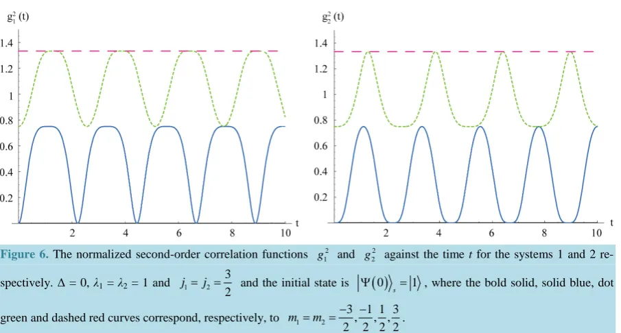
In Figure 6, we consider (Δ = 0, λ1 = λ2 = 1, 1 2 3 2
j = j = and the initial state is
( )
0 1s
Ψ = ). We investi-
gate the effect of the quantum numbers m1, m2 on the correlation functions g12 and 2 2
g for the systems 1 and 2 respectively. When 1 2 3
2
m =m =− , 2 2 1 2 0
g =g = , at any time, so in this case the functions show uncorrelated
behavior. When 1 2 1 2
m =m =− , the correlation functions 2 1
g , 2
2
g have regular and periodic oscillations and
2 2 1 2 1
g =g < , so in this case also the functions show uncorrelated behavior. When 1 2 1 2
m =m = , the correlation
functions 2 1
g , 2
2
g have regular and periodic oscillations, but in this case the functions sometimes show un-correlated behavior ( 2 2
1 2 1
g =g < ) and sometimes show correlated behavior ( 2 2 1 2 1
g =g > ) periodically. When
1 2
3 2
m =m = , 2 2 1 2 1.3
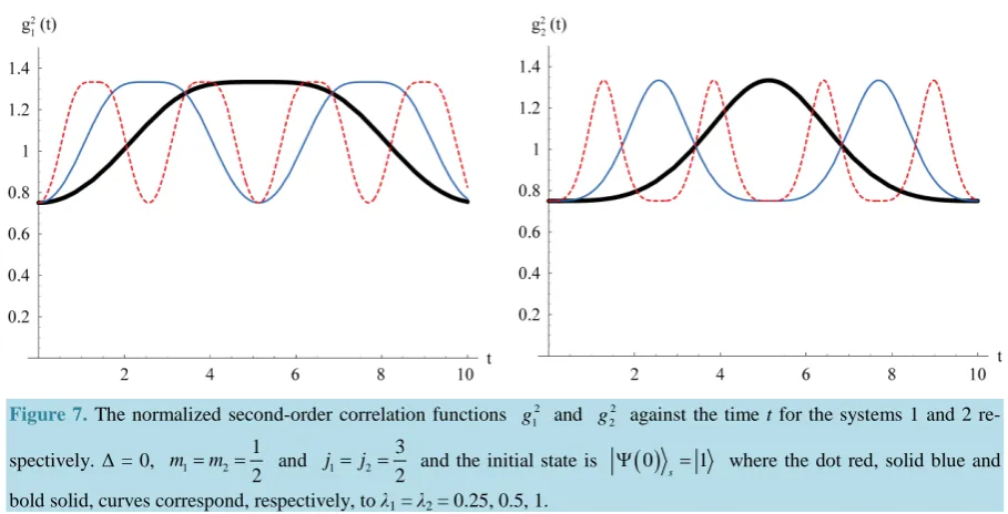
g =g = , at any time, so in this case the functions show correlated behavior. In Figure 7, we
consider (Δ = 0, 1 2 1 2
m =m = , 1 2 3 2
j = j = and the initial state is
( )
0 1s
Ψ = ). We investigate the effect of
the coupling parameters between spins λ1, λ2 on the correlation functions g12 and 2 2
g for the systems 1 and 2 respectively. The correlation functions 2
1
g , 2
2
g have regular and periodic oscillations, the functions some-times show uncorrelated behavior ( 2 2
1 2 1
g =g < ) and sometimes show correlated behavior ( 2 2 1 2 1
g =g > ) period-ically. When the coupling parameters between spins λ1, λ2 increase the number of periodic oscillations increases.
5. Conclusions
In this paper, we analytically solved the model that described the interaction between a three-level atom coupled to two systems of N-two level atoms. We calculated the atomic inversion and the Pancharatnam phase for some special cases of the initial states
(
( )
0)
s
Ψ , and special values of the quantum numbers m m1
( )
2 , the coupling parameters between spins λ1, λ2. The atomic inversion has regular and periodic oscillations. We observe, at the initial state( )
0 1s
Ψ = , when the quantum numbers m1, m2 increase, the phase of periodic oscillations gradu-ally decreases, until the phase of periodic oscillations reaches zero (straight line), but the minimum value in-creases until it equalizes the maximum value
(
)
max min 1
z z
S = S = (straight line). At the initial state
( )
1 1 10 1 2 3
2 2
2
s
Ψ = + + , the atomic inversion has small oscillations in the middle of the apexes of the
Figure 6. The normalized second-order correlation functions 2
1
g and 2 2
g against the time t for the systems 1 and 2 re-spectively. Δ = 0, λ1 = λ2 = 1 and 1 2
3 2
j = j = and the initial state is
( )
0 1 sΨ = , where the bold solid, solid blue, dot
green and dashed red curves correspond, respectively, to 1 2
3 1 1 3
, , ,
2 2 2 2
[image:9.595.89.542.477.720.2]
Figure 7. The normalized second-order correlation functions 2
1
g and 2 2
g against the time t for the systems 1 and 2
re-spectively. Δ = 0, 1 2
1 2
m =m = and 1 2
3 2
j = j = and the initial state is
( )
0 1 sΨ = where the dot red, solid blue and
bold solid, curves correspond, respectively, to λ1 = λ2 = 0.25, 0.5, 1.
oscillations when the quantum numbers m1, m2 increase, the number of periodic oscillations decreases and the small oscillations disappear gradually. We observe that there is constant interval at the maximum value. It in-creases remarkably when the coupling parameters between spins λ1, λ2 decrease and the number of periodic os-cillations gradually decreases. The Pancharatnam phase has regular and periodic straight lines following the shape of the letter N. We note that there is a regular repeat in the behavior of the Pancharatnam phase. When the quantum numbers m1, m2 increase and the coupling parameters between spins λ1, λ2 decrease, each period of the Pancharatnam phase widens on the time axe and the overall number of periods decreases. Comparing the change of the Pancharatnam phase in Figure 4 and Figure 5, we observe that the effect of the quantum numbers m1, m2 is larger than the effect of the coupling parameters between spins λ1, λ2 in respect to the overall number of pe-riods. Finally, we discuss the second-order correlation function where the examination of the second-order cor-relation function leads to better understanding for the nonclassical behavior of the system. When the quantum numbers m1, m2 increase the correlated behavior shows remarkably.
The model presented in this paper can further be applied to two-two level atom or two qubits where in this case j = 1. This can make contribution to more understanding and possible applications in the field of quantum optics as well as solid-state physics. In addition, the atom-atom (i.e. spin-spin) interaction is a promising candi-date for implementing the quantum computer, which accordingly can be connected vitally to the demonstration of spin dynamics in semiconductor structures [33].
Acknowledgements
I would like to express my deep gratitude to Professors Abdel-Shafy F. Obada, Mohamed M. A. Ahmed, De-partment of Mathematics, Faculty of Science, Al-Azhar University and Professor Mahmoud Abdel-Aty, Zewail City of Science and Technology, Giza, Egypt, for their support, care, their useful suggestions, useful discussion and for their continuous help and guidance.
References
[1] Mandel, L. and Wolf, E. (1995) Optical Coherence and Quantum Optics. Cambridge University Press, Cambridge.
http://www.cambridge.org/US/academic/subjects/physics/optics-optoelectronics-and-photonics/optical-coherence-and-quantum-opticshttp://dx.doi.org/10.1017/CBO9781139644105
[2] Walls, D.F. and Milburn, G.J. (1994) Quantum Optics. Springer, Berlin Heidelberg.
http://dx.doi.org/10.1007/978-3-642-79504-6
[3] Gardiner, C.W. and Zoller, P. (2004) Quantum Noise. Springer, Berlin Heidelberg.
[image:10.595.85.540.81.313.2][4] Moya-Cessa, H.M. and Soto-Eguibar, F. (2011) Introduction to Quantum Optics. Rinton Press, New Jersey.
http://www.rintonpress.com/books/0611.html
[5] Scully, M.O. and Zubairy, M.S. (1997) Quantum Optics. Cambridge University Press, Cambridge.
http://dx.doi.org/10.1017/CBO9780511813993
[6] Schleich, W. P. (2001) Quantum Optics in Phase Space. Wiley, Weinheim.
http://www.amazon.com/Quantum-Optics-Phase-Wolfgang-Schleich/dp/352729435X
[7] Kira, M. and Koch, S.W. (2011) Semiconductor Quantum Optics. Cambridge University Press, Cambridge.
http://dx.doi.org/10.1017/CBO9781139016926
[8] Agrawal, G.P. and Mehta, C.L. (1974) Dynamics of Parametric Processes with a Trilinear Hamiltonian. Journal of Physics A: Mathematical and General, 7, 607. http://dx.doi.org/10.1088/0305-4470/7/5/011
[9] Tucker, J. and Walls, D.F. (1969) Quantum Theory of Parametric Frequency Conversion. Annals of Physics, 52, 1-15.
http://dx.doi.org/10.1016/0003-4916(69)90318-2
[10] Tang, C.L. (1969) Spontaneous Emission in the Frequency Up-Conversion Process in Nonlinear Optics. Physical Re-view, 182, 367. http://dx.doi.org/10.1103/PhysRev.182.367
[11] Tucker, J. and Walls, D.F. (1969) Quantum Theory of the Traveling-Wave Frequency Converter. Physical Review, 178, 2036. http://dx.doi.org/10.1103/PhysRev.178.2036
[12] Walls, D.F. and Barakat, R. (1970) Quantum-Mechanical Amplification and Frequency Conversion with a Trilinear Hamiltonian. Physical Review A, 1, 446. http://dx.doi.org/10.1103/PhysRevA.1.446
[13] Sebawe Abdalla, M. and Ahmed, M.M.A. (2012) Some Statistical Properties for a Spin-(1/2) Particle Coupled to Two Spirals. Optics Communications, 285, 3578-3586. http://dx.doi.org/10.1016/j.optcom.2012.04.014
[14] Eleuch, H. and Bennaceur, R. (2003) An Optical Soliton Pair among Absorbing Three-Level Atoms. Journal of Optics A: Pure and Applied Optics, 5, 528. http://dx.doi.org/10.1088/1464-4258/5/5/315
[15] Setea, E.A., Svidzinsky, A.A., Eleuch, H., Yang, Z., Nevels, R.D. and Scully, M.O. (2010) Correlated Spontaneous Emission on the Danube. Journal of Modern Optics, 57, 1311-1330. http://dx.doi.org/10.1080/09500341003605445
[16] Abdel-Aty, M. (2002) Influence of Second-Order Correction to Rayleigh Scattering on Pancharatnam Phase in a Three-Level Atom. Modern Physics Letters B, 16, 319. http://dx.doi.org/10.1142/S0217984902003816
[17] Abdel-Aty, M., Abdel-Khalek, S. and Obada, A.-S.F. (2000) Pancharatnam Phase of Two-Mode Optical Fields with Kerr Nonlinearity. Optical Review, 7, 499-504. http://dx.doi.org/10.1007/s10043-000-0499-6
[18] Bhandari, R. and Samuel, J. (1988) Observation of Topological Phase by Use of a Laser Interferometer. Physical Re-view Letters, 60, 1211. http://dx.doi.org/10.1103/PhysRevLett.60.1211
[19] Wagh, A.G. and Rakhecha, V.C. (1995) On Measuring the Pancharatnam Phase. I. Interferometry. Physics Letters A,
197, 107-111. http://dx.doi.org/10.1016/0375-9601(94)00914-B
[20] Wagh, A.G. and Rakhecha, V.C. (1995) On Measuring the Pancharatnam Phase. II. SU(2) Polarimetry. Physics Letters A, 197, 112-115.
[21] Zhao, Y.-G. and Li, B.-Z. (1997) Quantum Phases of Pancharatnam Type for a General Spin in a Time-Dependent Magnetic Field. Chinese Physics Letters, 14, 801. http://dx.doi.org/10.1088/0256-307X/14/11/001
[22] Lawande, Q.V., Lawande, S.V. and Joshi, A. (1999) Pancharatnam Phase for a System of a Two-Level Atom Interact-ing with a Quantized Field in a Cavity. Physics Letters A, 251, 164-168.
http://dx.doi.org/10.1016/S0375-9601(98)00882-2
[23] Simon, B. (1983) Holonomy, the Quantum Adiabatic theoreM and Berry’s Phase. Physical Review Letters, 51, 2167.
http://dx.doi.org/10.1103/PhysRevLett.51.2167
[24] Facchi, P., Mariano, A. and Pascazio, S. (1999) Wigner Function and Coherence Properties of Cold and Thermal Neu-trons. Acta Physica Slovaca, 49, 677-682.
[25] Jones, J.A., Vedral, V., Ekert, A. and Castagnoli, G. (2000) Geometric Quantum Computation Using Nuclear Magnetic Resonance. Nature, 403, 869-871. http://dx.doi.org/10.1038/35002528
[26] Pancharatnam (1956) Generalized Theory of Interference and Its Applications. S.Proc. Ind. Acad. Sci, 44, 247. [27] Francisco De Zela, F. (2012) The Pancharatnam-Berry Phase: Theoretical and Experimental Aspects. In: Pahlavani,
M.R., Ed., Theoretical Concepts of Quantum Mechanics, Intech, 289. http://dx.doi.org/10.5772/34882
[28] Abdel-Khalek, S., El-Saman, Y.S. and Abdel-Aty, M. (2010) Geometric Phase of a Moving Three-Level Atom. Optics Communications, 283, 1826-1831. http://dx.doi.org/10.1016/j.optcom.2009.12.065
[30] Bhandari, R. (1989) Berry’s Phase and the Pancharatnam Angle-Some Recent Observations. Bulletin of the Calcutta Mathematical Society, 81, 496.
[31] Hariharan, P. and Roy, M. (1992) A Geometric-Phase Interferometer. Journal of Modern Optics, 39, 1811-1815.
http://dx.doi.org/10.1080/09500349214551881
[32] Masashi, B. (1993) Decomposition Formulas for Su(1, 1) and Su(2) Lie Algebras and Their Applications in Quantum Optics. Journal of the Optical Society of America B, 10, 1347-1359. http://dx.doi.org/10.1364/JOSAB.10.001347