Forecasting Electrical Energy Consumption for Malfunction Detection in Complex Technical Systems

2018 IX International Conference on Optimization and Applications (OPTIMA 2018) ISBN: 978-1-60595-587-2

Forecasting Electrical Energy Consumption for Malfunction Detection in

Complex Technical Systems

Anna TATARCZAK

_{, Łukasz WIECHETEK}

_{, Adam KIERSZTYN}

_,

`

Marek MEDREK

, and Jarosław BANAS

Maria Curie-Skłodowska-University, Lublin, Poland Lublin University of Technology, Poland

Corresponding author

Keywords: Data mining, anomaly detection, machine learning, Particle Swarm Optimization method,

short-term trend.

Abstract. _{Issues related to monitoring and detection of an unexpected or hidden malfunction in}

complex technical systems become more important since the complexity of technical installations grows and the remote installations, without human supervision are widely used in many branches of industry. In the proposed solution we use detailed information on electricity consumption provided by smart energy metering technologies for monitoring and anomalies detection purposes. As the data source, we use the teletechnical installations of the telco operator network, which consists of several hundred installations of various types, each created from many standardized components like power supply, battery, air conditioner, transmitter, etc. We build individual energy consumption model of each analyzed facility, which reflects daily cycles, weekly, monthly and seasonal fluctuations. For our simulations, we use the Particle Swarm Optimization method, which allows us to parameterize the model and estimate the expected energy consumption rate. The results of simulations show very good convergence with measurement data and allow for real-time malfunction detection.

Introduction

Increasing requirements for industrial systems, rapid development of monitoring and sensors technology and increasing data transfer speed and capacity create opportunities for system automa- tion, even for complex technical installations. In such complex automation systems, the remote operator often fails to get an overview of the current installation status, since the sources of data are connected and can influence each other or the data is spread over different subsystems [14]. Such complexity lead to an over-straining of the capability of monitoring and continues diagnosis of the particular components of the installation directly, in real time.

A possibility to cope with these challenges is the application of user support systems in the fields of process monitoring, anomaly detection, diagnosis, and optimization. A step into this direction is the usage of process models which are automatically learned from process data. Self- learning of process models from data leads to considerable simplification of model creation and configuration. Process models can be applied to several modelbased assistance functions such as visualization, diagnosis or optimization. Typical goals of such self-diagnosis approaches for complex

¸

1

2

*

and distributed industrial automation systems are the detection of anomalies and suboptimal energy consumption [5].

Traditionally, such self-diagnosis approach is based on fault-detection and fault-diagnosis and uses structural knowledge of sub-systems and components of the installation to identify the root cause of malfunctions [1]. Such structural knowledge is organized in system-level or component-level models [11] which allow for model-based diagnosis since a close correlation between anomalies on such levels and fault exists [16]. Another approach, in the detection of anomalies problem, involves assessing information about the behavior of the system, e.g. through the observation and prediction of energy consumption by subsystems in different phases of the complex installation. Modeling of the energy consumption in the particular, discrete system modes leads to model-based approach [15].

This paper proposes a PSO as a simulation-optimization approach to forecast electrical energy consumption for malfunction detection which is commonly encountered at big companies or facto-ries. Our model combines presented solutions and introduces several new improvements. As the indicator of the system health, we use the energy consumption values continuously registered by the smart energy meters (SEM) installed in individual locations of the analyzed systems. SEM are the devices that can read and relay the energy consumption at discrete time intervals and they are used as the data source in our, time history method for energy forecasting. Moreover, we don’t use any information about the structural organization of the observed system because most important in our model is the temporary system behavior in the sense of energy consumption. We also don’t group the systems or system modes because in our approach we build an individual, independent model for each monitored complex system. We use the energy consumption time history data and computational optimization method for assessing instantaneous prediction of energy consumption in the future. As the optimization numeric tool, we use the particle swarm optimization (PSO) method which is one of the most popular, nature-inspired meta-heuristic algorithm developed by James Kennedy and Russell Eberhart in 1995 [3] and is considered as a promising algorithm in solving various optimization problems in the field of science and engineering.

The main contribution of the paper are summarized as follows:

ˆ Issues related to monitoring and detection of unexpected or hidden malfunction are formal-ized as a constrained search problem. As a result, instead of using traditional methods which suffer from the time-consuming combinatorial complexity, PSO algorithm has been used and being researched in a new optimization area, namely the energy sector.

ˆ Power consumption minimization reflects daily cycles, weekly, monthly and seasonal fluc-tuations are taken into account. In addition to minimizing power consumption, very good convergence with measurement data is guaranteed.

ˆ A PSO-based algorithm is proposed, and its efficiency and suitability to parallel implemen-tation allow the anomaly detection to be done in real time. Furthermore, our work facilitates developing an efficient tool for energy usage prediction model as well as other optimization applications

The Modeling Framework Structure

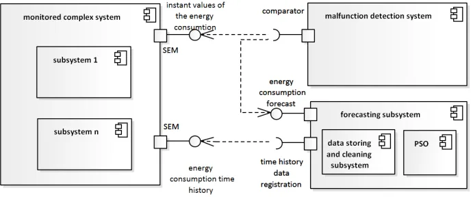
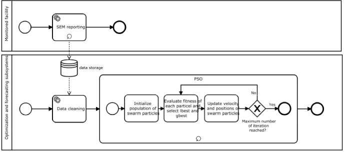
In our model we employ the PSO method for energy consumption forecasting based on time history data, collected by SEM at particular system location. Fig. 1 presents the component diagram of our modeling framework composed of three integral elements: data source, forecasting subsystem and malfunction detection system, which are described in sections 2.1, 2.2 and 2.3, respectively.

Figure 1. Component diagram of the modeling framework.

Since this paper focuses on the PSO method which we modify and adopt to the time history of energy consumption analysis, the other framework components are shown for illustration pur-poses only. The quantitative description of the PSO method, modified for malfunction detection purposes, is included in section 3.

Data Source Description – Monitored Systems

As the data source, we use the teletechnical installations of the telco operator network, which consists of several hundred installations of various types, each created from many standardized components like power supply, battery, air conditioner, transmitter, etc. For our purposes we build an individual energy consumption model for each analyzed facility. The input data are obtained from the SEM, therefore we limit modeling to facilities equipped with smart meters. The total, instantaneous energy consumption Eh

d in the facility is the amount of energy used by all its

components in the chosen period of time, described by following equation:

E_dh =

n

X

i=1

E_d,ih ,

where d and h are the date and daily hour of the analyzed instant of time respectively, i is the index of the facility component, n is the total number of components and E_d,ih denotes the power consumption by i-th component. The energy meter sends information about the total energy consumption in the cycle of δh hour incrementally, therefore for our purposes we calculate the differential energy consumption ∆E_dh in the analyzed period of time δhas

∆E_dh =E_dh−E_dh−δh.

Analyzing the available data, we choseδh= 1 hour as the base time resolution for our analysis. Moreover, we assume that such hourly energy consumption readings are available for at least a two-year period of time. Such a long period of observation is necessary to reflect the daily cycles, weekly, monthly and seasonal consumption fluctuations and remove the artifacts from the data.

Figure 2. Learning phase of the model.

Obtained values of ∆E_dh we use during the learning phase of our modeling scenario presented in Fig.2. This phase of modeling, using the PSO optimization algorithm, leads to the equation modeling the value of instantaneous energy consumption in individual objects, based on previous meter readings.

Particle Swarm Optimization Method – Forecasting Subsystem

The PSO is a heuristic bioinspired optimization algorithm that is well suited to solve high-dimensional and multimodal optimization problems [13, 9] and it is described in analogy with an activity of bird flocking or fish schooling, to find food or to escape from enemies, by splitting up into groups [4]. In PSO algorithm, bird is called a particle and its location represents a n-dimensional solution space is explored using a swarm of M particles, seeking to minimize an objective function f. The whole particle swarm flies in the search space to search for the global optimum, the best location corresponds to the particle whose objective value is the minimum among other particles. One round of observations from all particles corresponds to one iteration in the PSO. The neighborhood is determined by the used population topology: the lbest and the gbest topology [2, 10]. In the lbest swarm, only a specific number of particles can affect the velocity of a given particle. In the gbest swarm all the particles are neighbors of each other, and the position of the best overall particle in the swarm is used in the velocity update the equation [7]. If the stopping criterion is satisfied, the process stops and the final gbest is reported as the optimal population. The sub-process PSO in Fig.2 displays an illustration of the PSO algorithm. The cycle of seeking the new best position of each particle is iterated, to achieve the best solution.

Malfuction Detection System

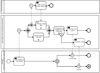
The goal of malfunction detection system is to discover symptoms indicating the difference between nominal and faulty status of the analyzed facility. In our approach, the instantaneous energy consumption time history is the parameter that characterizes the current installation oper-ation and its comparison with the short-term energy consumption forecast is the indicator of the correct operation of the facility (Fig.3).

Figure 3. The process model of the malfunction detection phase.

The process of the malfunction detection phase (Fig.3) is triggered by the operator of the malfunction detection system. In the next step, the operator sends the message to forecasting subsystem, where it starts the parallel tasks which generate the forecast and gather the current SEM reading for comparison purposes. If the forecast differs from the current indications, an escalation signal is generated, which is transmitted to the malfunction detection subsystem.

Since the daily course of energy consumption may take quite a different form for different categories of objects and within the individual categories significant differences may occur (both in the consumption values as well as in the shape of the function describing the energy consumption) we decided to determine the independent, individual forecast for each analyzed facility.

Time History Based Malfunction Detection Method

As was shown in section 2.3, correct determination of typical energy consumption patterns allows discovering potential failure of complex system, near in real-time (with accuracy toδh). The main part of our framework utilizes the PSO optimization, which leads to the formula modeling instantaneous energy consumption and the formula should be individually constructed for each analyzed object (due to the difficulty with the classification of the analyzed objects - see section

2.3). In the next subsections, it is described two approaches to forecasting energy consumption values. The first approach is based on the use of a moving average. The second approach uses a weighted moving average, in which the weight values are determined using the PSO method.

In order to simplify the notations (limit to only one facility), let xk

n for n = 0,1,2, . . . ,23 and

k = 0,1,2, . . . denote the differential value of energy consumption in the analyzed facility recorded

at the time n on thek-th day before the analysis with the time resolution δt= 1 h. For example, x4

5 means the energy consumption value recorded at 5 am, 4 days before the forecast.

A Model Based on Moving Average

The most obvious approach is to use a moving average. Based on the available data for the previous days, energy consumption is forecasted for the next period. For a given observation time n = 0,1,2, . . . ,23 it is proposed to use the mean given by the formula

¯

xM_n = 1

M

M

X

k=1

xk_n,

where M is the number of days that are taken into account. In order to estimate the quality the model we use the relative deviation error δn

δn =

x0_n−x¯M_n

x0 n

,

where x0

n denotes real value of energy consumption reading.

In the above model, every sum factor is taken into account with equal weight. Considering the slightly changed form of the model, with attention to different scales of individual factors of the sum, we receive the new definition of weighted average ˜xM

n :

˜

xM_n = 1

M

M

X

k=1

xk_n·ωk, (1)

where ωk _{≥ 0, k = 1,2, . . . are weights. In addition, we consider an acceptable errors for the}

average ¯xM

n and weighted average ˜xMn . Equation (2) and (3) define the error intervals for ¯xMn and

˜

xM_n , respectively

¯

xM_n −sn; ¯xMn +sn

, (2)

˜

xM_n −s˜n; ˜xMn + ˜sn

, (3)

wheresn,˜snare the standard deviations of ¯xMn and ˜xMn , respectively, given by the following formulas

sn =

q

1 M

PM

k=1(xkn−x¯Mn ) 2

, ˜sn =

q

1 M

PM

k=1(xkn−x˜Mn ) 2

.

Section 4 presents the numerical results for various types of facilities and different lengths M of the analyzed period. Moreover, we discuss also the different types of weights ωk _{used in the}

Generalized Model with Weighted Average

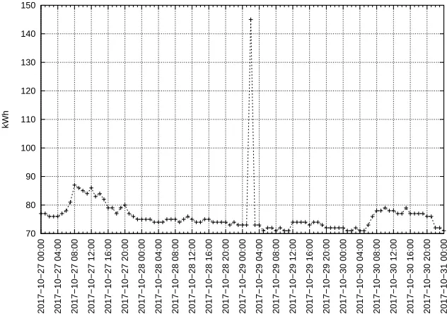
The models from section 3.1 take into account subsequent days, immediately preceding the forecast day. In result, it is impossible to reflect monthly or seasonal fluctuations in such models, e. g. the phenomenon presented in Fig. 4. The single peak of energy consumption visible at 2017-10-29, 2 a.m. will be treated as an anomaly, because considered models do not reflect longer trends and patterns.

70 80 90 100 110 120 130 140 150

2017−10−27 00:00 2017−10−27 04:00 2017−10−27 08:00 2017−10−27 12:00 2017−10−27 16:00 2017−10−27 20:00 2017−10−28 00:00 2017−10−28 04:00 2017−10−28 08:00 2017−10−28 12:00 2017−10−28 16:00 2017−10−28 20:00 2017−10−29 00:00 2017−10−29 04:00 2017−10−29 08:00 2017−10−29 12:00 2017−10−29 16:00 2017−10−29 20:00 2017−10−30 00:00 2017−10−30 04:00 2017−10−30 08:00 2017−10−30 12:00 2017−10−30 16:00 2017−10−30 20:00 2017−10−31 00:00

kWh

Figure 4. Energy consumption as a function of time.

In fact, the phenomenon presented in the Fig. 4 is not an atypical behavior, it occurs for all analyzed objects and it repeats every year for the same date and time. We notice that it is related to the winter time change when SEM doubles the value of energy consumption for the time at 2 a.m. In order to reflect such a long-term scheme we use the average ˙x0

n given by

˙

x0_n= a·

P7

k=1x n k+b·

P4

k=2x 7k

n +c·x7n·52

7a+ 3b+c ,

where a, b and c are the weekly, monthly and annual memory coefficients, respectively. In this model the cost function we define as the variance

s2_n = 1 11

" ₇ X

k=1

xk_n−x˙0_n2+

4

X

k=2

x7k_n −x˙0_n2+ x7_n·52−x˙0_n2

#

which should be minimized in three dimensional space (a,b, c).

Ultimately, it is possible to use the model with a more complex form of the weighted average given by

˙ x0_n =

PM

i=1 ωi·x ki

n

PM

i=1ωi

,

where ki is an increasing sequence of indexes i = 1,2, . . . , and ωi are the weights. As before,

weights should be chosen to minimize the variance (cost function) s2_n= _M1 PM

i=1 x ki

n −x˙0n

2

. It is impossible to solve such non-linear problem with relatively simple methods. Since the coefficientsa,b andccan take any real values from any range, it is advisable to use more sophisti-cated methods. One of the possible solutions is the use of the PSO method [8] described in section 2.2.

Figure 5. Position updates in PSO method [6].

In the PSO algorithm, the behavior of N molecules / objects / agents moving in the M -dimensional space is analyzed. Most often it is a coherent subset of the RM space. Each of the analyzed objects has information about its exact location x = [x1, x2, ..., xM], the direction of

motion v = [v1, v2, ..., vM], the value of the objective function for the current position, its current

best positionpbest= [p1, p2, ..., pM], values of the objective function for the best position, the best

position determined by all analyzed objects qbest= [q1, q2, ..., qM]. In the next steps, each object

determines its new direction of movement by formula

v =c1·v+c2·(pbest−x) +c3·(qbest−x) (4)

and a new location using by

x=x+v. (5)

Parametersc1, c2, c3 correspond respectively to the memory of its previous location, its impact on

the direction of its current best location, and the influence on the direction of the best location determined by the whole swarm( see Fig.5).

Numerical Results and Discussion

In this section, the team used real data on the electric energy consumption coming from a large telecommunications company. For the analysis, objects from four different categories of objects were randomly selected. Object A belongs to the group ”outdoor mobile container”, object B belongs to ”technical objects”, object C is an ”office and technical object”, while D is an ”outdoor FIX container”.

One of the key aspects when examining the quality of the proposed model is the proper selection of the parameters found in the formula (4). We will use the number of steps to achieve the optimal value for testing the efficiency (rate of convergence) of parameter selection. The c1 parameter is

c1 = 0.9−0.7·

number of iteration permitted number of iterations

In both approaches the rate of convergence, identified with the number of steps to achieve the optimal solution, is comparable and in the analyzed considerations of the value of the parameter c1 has no significant impact on the rate of convergence. For some objects, a faster average rate

of convergence with a constant coefficient is obtained, for others with a decreasing factor. The parameter c2 determines the force with which the object moves towards its previous best

posi-tion. It is usually assumed that this parameter has a uniform distribution on the interval [−a, a]. Similarly, c3, which determines the force with which an object moves towards the globally best

position, usually has a uniform distribution in the interval [−b, b] Convergence rate for different values of parameters a and b presents Table 1.

Table 1. Average convergence rate.

a\ b 1 2 3

1 371 495 445

2 518 517 455

3 571 410 515

As we can see, both parameters have a uniform distribution on the interval [−1; 1]. Otherwise, the algorithm needs more steps to achieve the optimal solution.

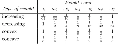
Different types of weights can be used in eq. (1). Four classes of weights were tested: increasing, decreasing, convex and concave. In the case of increasing weights, we assume that the more distant in time observations have greater weight. In the case of decreasing weights, there is a reverse relation. The values of the convex weights form a graph of the convex function. In all cases, the consecutive reversals of the power of number 2 are considered. The weight values for M = 7 are shown in the Table 2.

Table 2. Example values of weights used in eq. (1).

Weight value

Type of weight ω1 ω2 ω3 ω4 ω5 ω6 ω7

increasing ₆₄1 ₃₂1 ₁₆1 1₈ 1₄ 1₂ 1

decreasing 1 1₂ 1₄ 1_{8 16}1 ₃₂1 ₆₄1

convex 1 1₂ 1₄ 1₈ 1₄ 1₂ 1

concave 1₈ 1₄ 1₂ 1 1₂ 1₄ 1₈

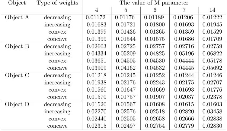
Median error values for decreasing weights for different object classes are shown in Figure 6. It turns out that the smallest error is achieved when energy consumption readings from the four preceding days are taken into account. This dependence remains correct regardless of the type of object. For all types of objects, a longer analysis period does not improve the results - the median error is almost constant for 6, 7 and 14 days. Median values of error for different types of weights and different test periods for sample objects are presented in Table 3.

Analyzing data from Table 3, it can be concluded that regardless of the type of considered objects and of the type of weights, the best results are obtained in the case of the average calculated for the period M = 4. Similar results show the average error instead of the median error. In the

0.010 0.012 0.014 0.016 0.018 0.020 0.022 0.024 0.026 0.028

4 5 6 7 8 9 10 11 12 13 14

median

days

object A object B object C object D

Figure 6. Median error for analyzed objects as a function of analysis time.

Table 3. Median model error

Object Type of weights The value of M parameter

4 5 6 7 14

Object A decreasing 0.01172 0.01176 0.01189 0.01206 0.01222

increasing 0.01683 0.01721 0.01800 0.01693 0.01945

convex 0.01399 0.01436 0.01365 0.01359 0.01529

concave 0.01399 0.01544 0.01575 0.01686 0.01709

Object B decreasing 0.02603 0.02725 0.02757 0.02716 0.02759

increasing 0.04334 0.05209 0.04825 0.05196 0.06822

convex 0.03651 0.04505 0.04530 0.04444 0.05178

concave 0.03909 0.04162 0.04532 0.04445 0.05692

Object C decreasing 0.01218 0.01245 0.01252 0.01244 0.01246

increasing 0.01938 0.02176 0.02243 0.02175 0.02707

convex 0.01560 0.01647 0.01669 0.01693 0.01776

concave 0.01570 0.01757 0.01907 0.02037 0.02378

Object D decreasing 0.01520 0.01567 0.01608 0.01615 0.01603

increasing 0.02270 0.02576 0.02518 0.02820 0.03458

convex 0.02440 0.02505 0.02658 0.02666 0.02838

concave 0.02315 0.02497 0.02754 0.02779 0.02830

above considerations, the median error is determined based on 31 days of observation. More specifically, we analyzed 24 SEM readings per day for 31 consecutive days. In result, the total sample item number is 744.

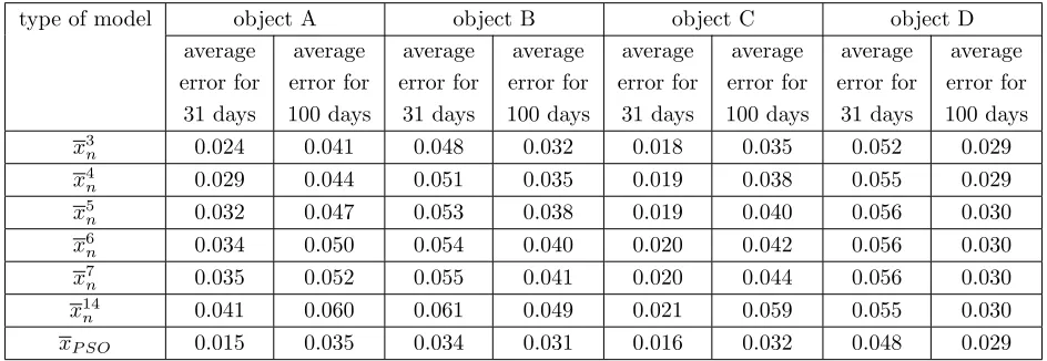
Table 4. Comparison of average error for different forecasting energy consumption method and various types of objects.

type of model object A object B object C object D

average error for 31 days average error for 100 days average error for 31 days average error for 100 days average error for 31 days average error for 100 days average error for 31 days average error for 100 days

x3n 0.024 0.041 0.048 0.032 0.018 0.035 0.052 0.029

x4_n 0.029 0.044 0.051 0.035 0.019 0.038 0.055 0.029

x5_n 0.032 0.047 0.053 0.038 0.019 0.040 0.056 0.030

x6_n 0.034 0.050 0.054 0.040 0.020 0.042 0.056 0.030

x7

n 0.035 0.052 0.055 0.041 0.020 0.044 0.056 0.030

x14

n 0.041 0.060 0.061 0.049 0.021 0.059 0.055 0.030

xP SO 0.015 0.035 0.034 0.031 0.016 0.032 0.048 0.029

that the error of the PSO method is smaller than for different optimization methods.

In the second case, in order to model the anomalies we produce distorted time series according to equation

∆E_dh,r2 = ∆E_dh+random(−0.5·∆E_dh; 0.5·∆E_dh),

where r2 = 1,2, .., n represents randomly chosen value of hours in the range r2 ∈ (2, n), for which we generate some artificial anomaly in energy consumption on d day of the real signal. The amplitude of the deviation was constant for the whole period and chosen according to the real anomaly detected by the teleco operator. We checked that for all analyzed objects, in 96.4% cases the PSO model detects the anomaly when the deviation from the real signal was bigger than 0.05·∆Eh

d and the period of registered anomaly was longer than 4 hours.

Conclusion

Currently, anomaly detection methods are of major interest to the world and are used in very different and various industry domains. In this paper, to the best of our knowledge, for the first time, the PSO algorithm was applied to the monitoring and anomalies detection problem in the teleco operator network, following two methods: weighted moving average and PSO optimiza-tion method. Furthermore, the proposed approaches were empirically compared using the teleco datasets. The experimental evaluation presented in this paper shows the satisfactory performance of our approach in terms of computational time and quality. Convergence of the proposed methods is studied for finding the optimal results in the training phase. In general, it can be found that in the second method better results are achieved to detect anomalies in the monitoring data.

This model can be used for short-term energy consumption forecasting or it can be a component of a larger anomaly detection system. There is ongoing research to improve our framework further. The model can be extended by adding more elements to the average and increasing the number of weights used during modeling. Finally, it would be also interesting to test the model in real conditions for a longer time interval to verify the correctness of its operation on identified anomalies cases. Future work will also aim to extend the approach for real-life applications.

Acknowledgements

The authors acknowledge the contribution of the industrial experts. This research has been fi-nancially supported by the Maria Curie-Sklodowska University Research Fund (Project: Incubator of innovation+ No. MNISW/2017/DIR/33/II+).

References

[1] L. Christiansen, A. Fay, B. Opgenoorth, and J. Neidig. Improved diagnosis by combining structural and process knowledge. In ETFA2011, pages 1–8, Sept 2011.

[2] Maurice Clerc. The swarm and the queen: towards a deterministic and adaptive particle swarm optimization. In Evolutionary Computation, 1999. CEC 99. Proceedings of the 1999 Congress on, volume 3, pages 1951–1957. IEEE, 1999.

[3] R. Eberhart and J. Kennedy. A new optimizer using particle swarm theory. InMicro Machine and Human Science, 1995. MHS ’95., Proceedings of the Sixth International Symposium on, pages 39–43, Oct 1995.

[4] Russell C Eberhart, Yuhui Shi, and James Kennedy. Swarm intelligence. Elsevier, 2001. [5] Rolf Isermann. Model-based fault-detection and diagnosis – status and applications. Annual

Reviews in Control, 29(1):71 – 85, 2005.

[6] Amin Karami and Manel Guerrero-Zapata. A fuzzy anomaly detection system based on hybrid pso-kmeans algorithm in content-centric networks. Neurocomputing, 149:1253 – 1269, 2015. [7] J Kennedy and R Eberhart. Particle swarm optimization. InIEEE International Conference

on Neural Networks (Perth, Australia), IEEE Service Center, Piscataway, NJ, pages 1942– 1948, 1995.

[8] James Kennedy. Particle Swarm Optimization, pages 760–766. Springer US, Boston, MA, 2010.

[9] James Kennedy and William M Spears. Matching algorithms to problems: an experimental test of the particle swarm and some genetic algorithms on the multimodal problem generator.

In Evolutionary Computation Proceedings, 1998. IEEE World Congress on Computational

Intelligence., The 1998 IEEE International Conference on, pages 78–83. IEEE, 1998.

[10] Tamer Mohamed Khalil, Hosam KM Youssef, and MM Abdel Aziz. A binary particle swarm optimization for optimal placement and sizing of capacitor banks in radial distribution feeders with distorted substation voltages. TM Khalil, HKM Youseef, MM Abdel Aziz, pages 129–135, 2006.

[11] Igor Mozetiˇc. Hierarchical model-based diagnosis. International Journal of Man-Machine Studies, 35(3):329 – 362, 1991.

[12] Jorge Pena, Andres Upegui, and Eduardo Sanchez. Particle swarm optimization with dis-crete recombination: an online optimizer for evolvable hardware. In Adaptive Hardware and Systems, 2006. AHS 2006. First NASA/ESA Conference on, pages 163–170. IEEE, 2006. [13] Yuhui Shi et al. Particle swarm optimization: developments, applications and resources. In

evolutionary computation, 2001. Proceedings of the 2001 Congress on, volume 1, pages 81–86. IEEE, 2001.

[15] S. Windmann, Shuo Jiao, O. Niggemann, and H. Borcherding. A stochastic method for the detection of anomalous energy consumption in hybrid industrial systems. In 2013 11th IEEE International Conference on Industrial Informatics (INDIN), pages 194–199, July 2013. [16] S. Windmann and O. Niggemann. Automatic model separation and application for

diagno-sis in industrial automation systems. In 2015 IEEE International Conference on Industrial Technology (ICIT), pages 1845–1850, March 2015.

[17] Yudong Zhang, Shuihua Wang, and Genlin Ji. A comprehensive survey on particle swarm optimization algorithm and its applications. Mathematical Problems in Engineering, 2015, 2015.