User assisted sparse stereo video segmentation

User-assisted Sparse Stereo-video Segmentation

Félix Raimbault, François Pitié and Anil Kokaram

Dept. of Electronic and Electrical Engineering Trinity College Dublin, Ireland

{raimbauf, fpitie, anil.kokaram}@tcd.ie

ABSTRACT

Motion-based video segmentation has been studied for many years and remains challenging. Ill-posed problems must be solved when seeking for a fully automated solution, so it is increasingly popular to maintain users in the processing loop by letting them set pa-rameters or draw mattes to guide the segmentation process. When processing multiple-view videos, however, the amount of user in-teraction should not be proportional to the number of views. In this paper we present a novel sparse segmentation algorithm for two-view stereoscopic videos that maintainstemporal coherence and

view consistencythroughout. We track feature points on both views with a generic tracker and analyse the pairwise affinity of both tem-porallyoverlappinganddisjoint tracks, whereas existing similar techniques only exploit the information available when tracks over-lap. The use of stereo-disparity also allows our technique to process jointly feature tracks on both views, exhibiting a good view consis-tency in the segmentation output. To make up for the lack of high level understanding inherent to segmentation techniques, we allow the user to refine the output with asplit-and-mergeapproach so as to obtain a desired view-consistent segmentation output over many frames in afew clicks. We present several real video examples to illustrate the versatility of our technique.

Categories and Subject Descriptors

I.4.6 [Image Processing and Computer Vision]: Segmentation

General Terms

sparse, motion segmentation, stereoscopic video, user interaction

Keywords

sparse, motion segmentation, stereoscopic video, user interaction

1.

INTRODUCTION

The recent revival of the stereo movie industry, as well as the slow infiltration of stereoscopic content in consumer market call for new

tools to automatise post-production tasks such as matte propaga-tion for compositing of stereo videos. A key technology to en-able the development of such tools isvideo segmentation, which has recently found many applications such as matting for cinema post-production [4], unsupervised learning [5], navigation for au-tonomous systems [1] and driver assistance systems [14].

Motion-based video segmentationaims at grouping together pix-els belonging to objects with asimilarmotion in a video sequence, following Gesalt psychology principles that try to explain how hu-mans perceive a coherent organisation of objects in a noisy world [20]. Defining what is an object is not trivial and each object could be represented by one or severalclustersof pixels. For instance an articulated object (e.g. an actor) could be segmented into sev-eral parts exhibiting different motions (e.g. head, arms, torso) as illustrated in figure 1. This problem is known as setting thelevel

of segmentation. Fully automated segmentation techniques [2, 27] need to infer the number of objects in the scene. However this is an ill-posed problem as the desired segmentation level ultimately de-pends on the application. Therefore, instead of segmenting a scene at a fixed level, a versatile technique would ideally output a hierar-chyof clusters so that the level of fragmentation can be increased or decreased by users, depending on their needs.

It is important that each identified object consistently belongs to the same cluster along the whole video, i.e. that the segmentation istemporally coherent. Otherwise, manual corrections of the video segments would be required in a later stage. But it is still chal-lenging for many state-of-the-art techniques to maintain a coher-ent grouping of pixels over many frames in real videos. In such sequences, lighting changes, object occlusions, complex camera motions and sensor noise are very common. These phenomena are challenging problems formotion estimationandfeature point tracking[24, 25] which are at the core of most video segmenta-tion algorithms. However, the most promising techniques enforce

long-term temporal coherenceby means of feature point trajecto-ries or tracks to obtain asparse representationof objects in the scene which span many frames [4, 5]. After generating point tra-jectories, the first step towards segmentation is to gather similar tracks together into clusters as illustrated in figure 1.

be-tween views arise inbinocular half-occlusionareas which are hid-den in only one view and should be segmented coherently with respect to the rest of the pixels. Besides, depth information that can be extracted from stereo pairs offers additional cues which can be combined with position, motion and colour to improve the quality of segmentation techniques [7, 14]. A general issue with segmen-tation is that it is an under-constrained problem, but the addition of depth or disparity-based constraints opens new possibilities that have not been explored that much in the literature so far.

The final goal of stereo-video segmentation is to assign every pixel to a cluster, i.e. generate adense segmentation of every frame. However,temporal coherenceandview consistencyconstraints must be enforced. Obtaining a sparse representation of a monoscopic video with feature trajectories has been employed as a first step to dense segmentation [4, 15, 17]. This allows exploitation of rich, long-term object position constraints and motion models that can be obtained from sparse video segments to yield a dense segmenta-tion in a two-stepsparse-to-denseapproach. This approach seems very promising to enforce temporal coherence and overcome limi-tations due to analysis at local level in state-of-the-art dense video segmentation techniques [1]. Moreover, it should benefit from the addition of stereo cues to enable joint processing of a stereo se-quence. Along these lines, we present in this paper a sparse stereo-video segmentation technique that can be employed as a stepping stone for dense stereo-video segmentation.

Our contributions: We propose a novel sparse stereo-video seg-mentation technique that builds up on the framework of Brox and Malik [5]. It extends it with a novel affinity measure ontemporally disjointtracks whereas state-of-the-art methods [12, 15] can only comparetemporally overlappingtracks. We show that our tech-nique increasestemporal coherenceof the output, enabling connec-tion of objects even after full occlusion if their moconnec-tion remains sim-ilar. Secondarily aconsistent segmentation across viewsis yielded by processing jointly tracks generated on both left and right views in a single framework, making use of disparity-based constraints. To the best of our knowledge, this aspect has not been investigated in the sparse video segmentation literature heretofore. Finally we propose auser-assisted split-and-merge methodallowing users to explore ahierarchyof clustersin a few clicksto generate an output with the level of segmentation that suits their needs without further processing. A binary tree of clusters in which each node represents a split step is obtained automatically beforehand by using a combi-nation of algorithms employed in state-of-the-art techniques.

Organisation of the paper:Section 2 reviews previous similar ap-proaches to sparse video segmentation. Section 3 details our tech-nique for sparse segmentation of stereoscopic videos. The novel affinity allowing to compare both overlapping and disjoint tracks in stereo videos is presented in Section 3.2. The automatic hierarchi-cal clustering method is described in section 3.3 before we present the user-assisted split-and-merge method in section 3.4. Experi-mental results are shown in section 4 before we conclude the paper.

2.

RELATED WORK

Exploitinglong-term point trajectoriesseems to be the most promis-ing way of obtainpromis-ing long-termtemporally consistentclusters. In-deed, faster (or even real-time) techniques [1], based on frame-to-frame propagation/relaxation usingOptical Flowhave troubles dealing with partial occlusions, spatially disconnected objects and large displacements. On the other hand, bottom-up segmentation

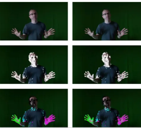
Figure 1: Sparse stereo segmentation on a stereo pair of frames from thegreen_screensequence. Feature points on the ac-tor can form a single cluster (middle row) or several clusters corresponding to different motions (bottom row).

techniques [5, 19, 27], which are based on the analysis offeature point tracks, need to employ a tracker (such as KLT [24], LDOF [25], PV [22], or VT [3]) to generate trajectories as a preprocess-ingstep. Not all feature point trackers perform equally in terms of spatial density and track length, but they all allow longer-term accurate correspondences between points than Optical Flow field.

Within a subclass of these track-based techniques, namelymanifold clustering, completeness of all [27] or some [19] of the tracks is a common assumption. But in practice feature point trackers yield trajectories of variable lengths, that can be corrupted by noise; key points disappear and reappear due to occlusions, new objects en-tering the scene as well as illumination and viewpoint changes. To mitigate these problems, some techniques [5, 12, 15] propose to analyse tracks by computing theirpairwise affinity(i.e. measuring howsimilartracks are to each other) during theirtime of overlap

thereby allowing tracks of varying sizes to be clustered efficiently. Once pairwise track affinity computed, many techniques [5, 27] employ spectral clustering algorithms [11, 23] that analyse the eigenvalues of theaffinity matrixto form groups of similar tracks. Otherenergy minimisationtechniques based on track affinities can be used [15]. These methods can deal with partial occlusions and tracking loss but break down fully occluded objects. A track repair mechanism [21] would be needed to connect temporally disjoint butsimilartracks. Bridging the gap between track repair and clus-tering, we propose to compute affinities for bothdisjointand over-lappingtracks to mitigate problems with fully occluded objects in state-of-the-art sparse video segmentation techniques.

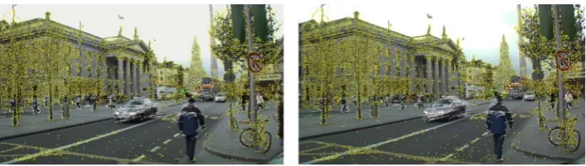
Sim-Figure 2: Bi-layer separation on a stereo pair from thegpo_fixedvideo. Points in yellow are ignored in subsequent segmentation.

ilarly, Fragkiadaki et al. [12] add a term based on themaximum stereo-disparity differencebetween tracks in one view of a stereo video alongside the maximum velocity difference. Occlusion rea-soning in the form of depth ordering constraints has been added to the pairwise affinity framework [15] to further constrain the prob-lem. However depth ordering is assumed constant over the video. We exploit stereo disparity as a more flexible natural depth ordering constraint for stereo videos [9, 12]. Our technique is also able to compare two trajectories that do not lie in the same view by adding corresponding disparity offsets to tracked feature point positions.

A common problem in most techniques is the lack ofhigh level un-derstandingof a video scene.Two-granularity tracking[12] com-bines thebottom-upapproach of Brox and Malik [5] with a top-downmodel-driven technique to track pedestrians in crowded en-vironment. The finer granularity of point tracks allows refinement of the model-based technique in case partial occlusions occur. Bal-ancing cues such as appearance and geometry [2] or colour and depth [7] can prove very hard and need manual tuning. In Baugh and Kokaram [4] the user is asked to draw a matte every ten frames to provide higher level information on the colour and motion of objects of interest. Parameter tuning can be time consuming and frustrating for the user, so we have tried to make most parameters

adaptive. However we ask users to choose the desired level of seg-mentation that fits their needs which only requires a few clicks.

Determining thenumber of clustersin the sequence is a difficult problem that requires high level understanding of the scene as well. Many automatic solutions have been proposed, exploiting spatial regularity [5], theAkaike Infomation Criterion[2], distribution of the model hyperparameters [13], spectral graph theory [27], etc. But none can predict what is the actual number of clusters desired by the user, which is application-dependant (e.g. only two clusters are necessary for foreground/background separation [14]) so it may be more practical to let the user set it as a parameter [15]. In some applications, however, over-segmentation is acceptable as long as it provides long-term associations between points while respecting object boundaries, so that the number of clusters need not to match exactly the number of objects in the scene. Our approach to that problem is to generate a hierarchy of clusters that can be navigated by the user to obtain the required segmentation result.

Reviewing in details howsparse-to-denseapproaches [4, 15, 17] turn clusters of tracks intodense video segmentsis out of the scope of this paper as we present a sparse segmentation technique. Inter-ested readers can refer to the provided references for further infor-mation. Now we have reviewed the current state of the art ofsparse video segmentation, the next section delves into details of our

ap-proach to solve thesparse stereo-video segmentationproblem.

3.

PROPOSED SOLUTION

This section details the steps of our sparse stereo-video segmen-tation technique. Firstly, section 3.1 explains the preprocessing

stages necessary to obtain a 6D feature vector at each tracked points in the whole stereo sequence and how static background points are discarded from further processing. Thesefeature point tracksare the input of the sparse segmentation algorithm per se. Section 3.2 shows howpairwise affinity scoresare computed between pairs of bothoverlappinganddisjointtracks in left and right views. Then section 3.3 describes thedivisive-agglomerative algorithmto gen-erate ahierarchy of clustersvia over-segmentation usingspectral clusteringbefore an agglomerative stepmerges pairs of clusters one by one. Finally section 3.4 explains how it is then expanded and refined during auser-assisted split-and-merge stepwhich al-lows users to select the desired level of segmentation of the output.

3.1

Preprocessing

Our method uses a sparse representation of a stereo video obtained viafeature point trackinganddisparity estimation. The idea is to store2D positionandstereo-disparityinformation, as well as their temporal derivatives for each feature point along their trajectory. Thus we obtain a 6D feature vector at each point by combining cues on positionXand velocityV:

F=



  

x,y,d

| {z } X

,∂x

∂t,

∂y ∂t,

∂d ∂t | {z }

V 

  

(1)

Following Gesalt psychology principles we seek to cluster together

proximatepoints exhibiting asimilar motion, following the frame-work of previous techniques [5, 12] and exploit the feature vectors

Fto computepairwise affinitiesbetween tracks (see section 3.2).

We employ the KLT feature tracker [24] on both views indepen-dently and off-the-shelf state-of-the-art disparity estimator avail-able inOcula1, a stereo software suite for a compositing software for movie post-production,Nuke2. We also estimate local Optical Flow fields withNuketo discard the most noisy KLT tracks that ex-hibit a drastically different displacement from corresponding local motion vectors. A stereo feature tracker [16] that simultaneously tracks points in both cameras could also be used advantageously in our technique, except that no points would be tracked on binocular half occlusion areas (i.e. points visible in one view only).

Information about 2D positions of tracked points is extended with their stereo-disparity information to form a 3D feature vector noted

X. We thus obtain a 3D representation for each point similar to Duan et al. [9]. We use it to favour grouping together points within a depth layer in our clustering algorithm (see section 3.3), as dis-parity is inversely proportional to the depth of the underlying 3D point. The position of a feature point can be inaccurate and wander across depth layers, causing spurious fluctuations of the disparity value. So we apply a temporal median smoothing filter on the dis-parity values along trajectories, using the previous and next frames.

Temporal derivatives of the position (i.e.velocity) and of the dispar-ity (that we calldepth variation) are then computed and denoted as a 3D feature vectorV. The 2D velocities are further processed to remove the influence of the camera motion noise. This step is sim-ilar to the use of video stabilisation in the track repair technique [21]. Indeed velocities oftemporally disjointtracks must be com-parable in the measure we detail in section 3.2, which would not be the case if they were corrupted by motion jitter (e.g. when the camera is handheld). Our procedure estimates aDominant Motion Vector[18] at each frame, on velocities of feature points only. It is then subtracted from all velocity values, on each view separately. Finally the corrected velocities and depth variation values are tem-porally smoothed out with a two-pass (forward and backward) one-tap IIR filter with parameterαM=0.75 to increase robustness in

subsequent computation involvingV.

Once velocities registered and smoothed, basicbi-layer segmenta-tionis used to label points that are moving due to camera motion as

background(see figure 2). These points have a computed velocity of 0 as velocities are registered to the camera motion. So we can de-tect them by a simple thresholding of the quantity of motion along time. If the maximum of theirsquared motion amplituderemains belowθM=2 along the trajectory, we classify the track as

belong-ing to the background. Staticbackground tracksare discarded in further processing as we are mainly interested in segmenting dy-namic objects. However we do not discard any tracks if the amount offoregroundtrajectories is less thanPM=50% of the total num-ber of tracks. This avoids inaccurate background labelling, which can happen under camera zooming, as our motion registration step is translational only. The bi-layer pre-segmentation step is useful to reduce computation speed and balance the size of clusters (the pres-ence of a very large cluster can bias some clustering techniques).

In section 3.2 pairwise affinities are computed between each and every pair of tracks,regardless of the view in which they reside. To enable that computation, a key point of our technique is computing of aview counterpartposition vector for each point:

X0= (x+d,y,−d) (2) The counterpart velocityV0stems fromX0as explained previously. GivenFandF0at each tracked point we can explain in details how affinity values between non-static tracks are computed and gathered in anaffinity matrix.

3.2

Computation of the Affinity Matrix

F0= (X0,V0)as explained in section 3.1. From now on, for nota-tional simplicity we note all feature vectors without prime regard-less, but assume that when given a pair of tracks(i,j)residing in different views, one of the tracks (e.g. the first one, i) uses itsview counterpartfeature vectorF_i0. For every tracki, the corresponding feature at frametis then notedF_it= X_it,V_it

.

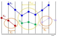
Figure 3: Affinity is computed on both overlapping (e.g. 1 and 2) and disjoint tracks (e.g. 3 and 4).

As stated in section 2, previous methods compute the pairwise affinity betweenoverlappingtracks(i,j), using feature vectors taken at framest∈Ti,j for which both tracks exist (e.g. tracks 1 and 2

in figure 3 are overlapping during 3 frames). A key novelty of our method is to compute affinities between disjointtracks(i,j) as well, using feature vectors taken at the extremity of each track. If trackistops before track jbegins, we use features at frames in setsT_i+at the end of trackiand inT_j−at the beginning of trackj. ConverselyT_i−andT_j+are employed if track jends before tracki

begins (e.g. tracks 3 and 4 in figure 3 are disjoint). IfTi,jcovers less

than two frames, we consider the tracks as being disjoint. We use

∆T=3 frames at the extremity of disjoint tracks. Whenever a track

is shorter than∆T, only the smallest amount of available frames is

considered in a pairwise computation involving this track.

3.2.1

Pairwise Distance Matrix

Following the framework presented in previous works [5, 15, 27] we perform track clustering on apairwise affinity matrixindicating howsimilartracks are to each other. The affinity matrix is derived from a pairwise normalised distance matrixDmade of two terms:

D(i,j) =

1+Ds(i,j)−ms

σs

Dt(i,j)−mt

σt

(3)

For all pairs of tracks(i,j). The matrixDsis the spatial pairwise distance andDtis the temporal pairwise distance. The normalising termσuforu∈ {s,t}is computed as the standard deviation of all

elements in the corresponding matrixDu excluding the diagonal. Similarlymuis the minimal value inDu. We found that automated normalising step to work well for all the sequences we have tested. Pairwise track distances can only compare the compatibility of tra-jectories on the basis oftranslational motion models[5], valid only for points that are close enough in space. To reduce the effects of that approximation we normalise the distance usingDsso that only proximate points can generate high affinities. One is added to the leftmost term so that when the normalised spatial distance is null, a low distance is obtained only if the temporal distance is low.

3.2.2

Spatial distance

The pairwise spatial normalisation termDs(i,j)in equation (3) is computed as follows:

Ds(i,j) =

(

µTi,j Xi−Xj

, if|Ti,j| ≥2

µT

a

i(Xi)−µTjb(Xj)

, otherwise.

(4)

We define the mean function asµT(X) =_|T|1 ∑t∈TXtand|T|as the

3.2.3

Temporal distance

The pairwise temporal distance termDt(i,j)in equation (3) is com-puted as follows:

Dt(i,j) =

  

 

maxt∈Ti,j

V

t i−Vtj

, if|Ti,j| ≥2

µ_Taa i(Vi)−µ

a Tb

j

(Vj)

, otherwise. (5)

Whereaandbare defined as in equation (4). The average function

µ−excludes one frame at the beginning of a track as the velocity

is not defined on the first frame, but considers the∆T following

frames. Andµ+is the same asµ. The distance enforces the for-mulation of Brox and Malik [5] for overlapping tracks, with the addition of thedepth variationterm. Moreover, high affinity is as-signed to disjoint tracks which exhibit a similar motion on average at their extremities. Note that onlystationarydisjoint tracks would legitimately have a high affinity in our formulation. It is important to repeat that the values computed for disjoint tracks assume that the effects of camera jitter are removed in the velocity terms (see section 3.1), following the track repair framework [21].

3.2.4

Temporal decay

The approximation of stationarity made in equation (5) for disjoint tracks holds only for tracks that are not too far apart in time, so we define a decay factorλto lower the affinity of disjoint tracks as the

length of the temporal gapgi,jbetween them widens:

λ(i,j) =

 



1, if|Ti,j| ≥2

exp

−g2i,j 2σt2

, otherwise. (6)

Whereσtequals the number of frames in the sequence, as we have

obtained better results when not constraining the value too much.

3.2.5

Pairwise Affinity Matrix

The affinity matrixAis computed as a mixture of a distance-based affinity matrixAD computed fromD, and a neutral value µD to

which disjoint tracks that are far apart converge:

A(i,j) =λ(i,j)AD(i,j) + (1−λ(i,j))µD (7)

WhereAD(i,j) =exp(−D(i,j)2_{)withDfrom equation (3). And}

µDis the mean value of the elements inADcorresponding to

over-lapping tracks only, excluding the diagonal. Then affinity values are normalised to[0,1]. The mixing weightsλare the decay values for disjoint tracks from equation (6). This ensures that more credit is given to affinities of disjoint tracks that are not too far apart in time while mitigating more dubious values (viz. when tracks are far apart in time) with a neutral scalar computed from more reli-able affinities of overlapping tracks. Note that the average of val-ues obtained by comparing both left-to-right and right-to-left view counterpart tracks is assigned to the final values inDsandDt con-stituting the distance matrixD.

We have now explained in detail how to compute affinity values between all pairs of tracks. In section 3.3 we move on to the seg-mentation algorithm which uses that information to form groups of clusters and show that the output respects bothtemporal coherence

andview consistencyconstraints mentioned in section 1.

3.3

Divisive-Agglomerative Clustering

This section describes how we construct a hierarchy of track clus-ters via adivisive-agglomerativeclustering approach [2]. The di-visivestep uses spectral clustering withNormalised Cuts[23] on

Figure 4: Output of divisive step of section 3.3.1 on the

gpo_track_2sequence (details). Using affinity on both over-lapping and disjoint tracks allows recovery from full occlusion.

the pairwise affinity matrix computed as explained in section 3.2 to

over-segmentthe stero video and produce a large number of small but consistent clusters and the followingagglomerativestep uses

Min-max Cutlinkage [8] to merge all clusters one by one, thereby forming a binary tree where each node corresponds to a split move when reading the tree from the root.

3.3.1

Divisive Step

Once the pairwise affinity matrixAcomputed for all pairs of tracks, we analyse its eigenvalues to find clusters of tracks. Dal Mutto et al. [7] compare several clustering algorithms to segment stereo im-ages using geometry and colour. They found that the most reliable and efficient technique on their data is spectral clustering with the Nyström method [11]. It is an approximation to solve the eigen-function problem ofNormalised Cuts[23] more efficiently, making it scalable to process big datasets. In our experiments we used the

recursive two-way Ncut algorithm [23] with a modified stopping criterion for a better control on the size and coherence of the clus-ters. Thisdivisive stepyields an over-segmentation of the tracks, generating small but very consistent clusters.

Thetwo-way Ncutalgorithm [23] boils down to thresholding the eigenvalue corresponding to the Fielder vector associated with the second smallest eigenvalue of the normalised Laplacian matrix de-rived from the affinity matrixA. Thereby it finds a splitting point that optimally partitions the underlying graph in two. Each sub-graph is then sub-partitioned iteratively until a stopping criterion is reached. It is hard to attach a physical meaning to the original cri-terion [23]. So we adopted a more pragmatic approach that directly controls the coherence of the clusters in terms of affinity values. First we define the binary matrixBwhich locates pairs of tracks with low affinities that should not be grouped together:

B(i,j) =

(

1, ifA(i,j)≥θA

0, otherwise. (8)

Where the thresholdθAgives an indication on what is ahigh

affin-ity value. We defineθAas the mean value of values of A greater that

Figure 5: Output of divisive step of section 3.3.1 on the

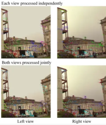
building_sitesequence (details). The shape of the clusters differ significantly on the top row (in the right area especially) and are much more consistent on the bottom row.

nk in the current cluster under scrutiny is greater thannmin=3, we pursue the partitioning of the weighted sub-graph only if the amount of confident pairs of tracksβk= nk(nk−11 )∑i6=jBk(i,j)is

greater than a thresholdθH=0.2, whereBkstores the values of Bfor the sub-graph. Finally small clusters which sizes are lesser or equal tonminare put together and the algorithm is run on that

sub-graph once more, to try and merge them back together.

We have compared the output of the divisive algorithm when using affinities on overlapping tracks only and all tracks and found out thattemporal coherenceis improved with the latter approach. As can be seen on figure 4 recovery from full occlusion is only pos-sible if disjoint tracks can yield a high affinity value as well. We also tried to run the divisive clustering on each view of a stereo video separately and compared it with our joint approach. As illus-trated in figure 5 the shape of clusters can differ significantly from one view to the other when processed separately whereas a much greaterview consistencyis attained by our approach.

3.3.2

Agglomerative Step

At the end of the divisive step we separate clusters that are disjoint in time. The following agglomerative step uses theMin-max Cut

linkage technique [2, 8] to iteratively merge all clusters together. At each iteration the algorithm merges the clustersCpandCqthat yield the greatest linkage score:

L(p,q) = S(p,q)

S(p,p)S(q,q) (9)

WhereS(p,q) =∑i∈Cp,j∈CqA(i,j)denotes the similarity between

clusters. The output of our clustering method is then a hierarchy of consistent clusters that can be represented as a binary tree in which each node corresponds to a split step, when reading from the root.

It is difficult to set an appropriate fixed level of segmentation cor-responding to a defined amount of split steps when traversing the tree. Therefore we ask the user to explore possiblesplit moves

beforemerging back some clusters. This user-assisted split-and-merge step is explained in section 3.4 before application of the technique is shown on examples in section 4.

3.4

User-assisted Split-and-Merge

Up to now we have not defined the number of clusters in the final output of our technique. As stated in section 2 defining automat-ically the appropriate number of clusters is a challenging problem for which a variety of ad-hoc solutions have been proposed. In fine the desired number of clusters isapplication-dependant(e.g. foreground/background segmentation requires two clusters, matte propagation can only require one or several specific object(s) to be segmented out of the rest of the sequence) so we have decided to let the user choose a suitable level of segmentation.

Determining a fixed level at which the tree defined in section 3.3 is pruned as in Angeli and Davison [2] can generate a solution that is not optimal for the purpose of the user, i.e.overorunder -segmented. Remember that the track comparison method we em-ploy is only able to model translations. The linkage measure we use for grouping in section 3.3.2 can then generate spurious associ-ations, for instance under heavy camera rotation around the optical axis where the local motion of tracks at the centre of the scene dif-fers drastically from the motion of tracks at the edges.

Therefore we propose to provide users with aninteractivetool that allows them to explore the clustering hierarchy to correct under or over-segmentation errors and reach the output that suits their needs. The technique can be implemented as a graphical user interface en-abling users to play back the video while refining the segmentation. Oneclickon a marker at the centroid of a cluster at a given frame would allow tosplitit in two, along all its duration and on both views until there is no under-segmented clusters remaining (see the output of the split step in the top row of figure 6), and a selec-tion toolwould then allow the user to click on several cluster to be merged together (see the output of the merge step on the bottom row of figure 6). If dense segmentation is desired, sparse segmentation can be used as a preview of the final output that can be generated in a fraction of the time required for a dense result.

In our tests we have implemented the technique as a command line tool, but in section 4 we refer to the number ofclicksand selec-tionsmade to segment a scene as an indicator of the amount of user interaction needed for a given segmentation task.

4.

EXPERIMENTS AND RESULTS

Now we have explained how our technique works we analyse user-assisted segmentation results on a few sequences extracted from a stereo-video database available online [6]. We keep 100 frames for every sequence in our tests. We also show the misclassifica-tion score of our automatic method applied to theHopkins 155

dataset [26] compared to two state-of-the-art sparse segmentation techniques. For all our tests we have used the parameter values as given throughout section 3. Videos corresponding to the results presented here as well as additional sequences can be viewed on our website athttp://www.sigmedia.tv/Misc/SSVS2013.

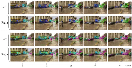
com-Figure 6:trafficsequence – user-assisted output after 7 split steps (top rows) and after 3 merge steps (8 selections) (bottom rows).

pared to two recent methods [10, 19]. On thetrafficand articu-latedsequences our results are in par with state-of-the-art scores but some sequences with heavy rotation of the camera among the

chequerboardsequences obtain a very poor score, because the ag-glomerative step produces erroneous associations, as explained in section 3.4. There are many such sequences in that database, so the overall score suffers from that problem. It would be interesting to test our technique on the database presented in Brox and Malik [5] for tracks of variable lengths, which we plan to do in the future.

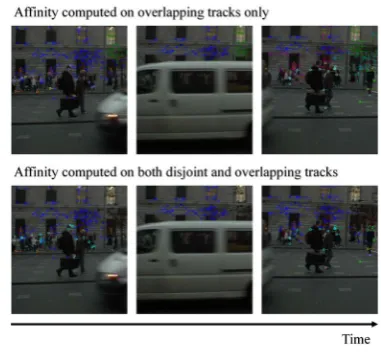
In figure 7 we show the output of automatic clustering presented in section 3.3, with the number of clusters set to 5. When com-puting affinities on overlapping tracks only, we set the affinity of non-overlapping tracks to 0 which indicates the lack of informa-tion regarding their associainforma-tion [12]. When computing the affini-ties on both overlapping and disjoint tracks with our novel affinity measure it can be seen that the segmentation is much more tempo-rally coherent. We also show on that example points estimated as background during preprocessing in gray.

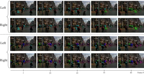
The next three figures compare the output of our automatic divisive-agglomerativealgorithm with a set number of clusters to the out-put obtained byuser-assisted explorationof the cluster hierarchy described in section 3.4. The examples are presented in increas-ing order of difficulty in terms of required user interaction. In the video presented in figure 8 motions of the tracks on the walking person and the rotating sphere are locally similar, causing wrong associations between the two objects, even though differences in position and disparity allows for separation of most of the tracks. Splitting the spurious clusters allows to efficiently differentiate be-tween the two objects. In the sequence presented in figure 9, vari-ations in the speed of the camera undergoing a panning movement causes the motion of points in the background to differ significantly over time and therefore to be over-segmented. User-assisted explo-ration allows to merge those points in one cluster and differentiate

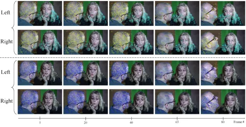
between the various moving objects in the scene. Finally the se-quence shown in figure 10 contains two main challenges. Firstly it is difficult to separate the background from the head of the actor, as both are immobile for a long period of time, and many tracks are terminated when he starts moving his head. Secondly the area in between both actors is problematic as they are close to each other and keep the upper-part of their torso almost immobile as well. User-assisted exploration, necessitating to over-segment the area connecting both actors ultimately allows to generate a meaningful segmentation separating both actors and the background. In all se-quencesview consistencyis enforced very well, so that in our tests the user never had to connect clusters residing in different views.

Figure 7:kylemoresequence – results of automatic divisive/agglomerative clustering with number of clusters set to 5, with over-lapping affinities only (top rows) and both overover-lapping and disjoint affinities (bottom rows).

2 motions 3 motions

sequences method ALCsp[19] SSC [10] our method ALCsp[19] SSC [10] our method

chequerboard mean 1.49 1.12 12.47 5.00 2.97 14.46

median 0.27 0.00 0.13 0.66 0.27 15.94

traffic mean 1.75 0.02 0.29 8.86 0.58 1.48

median 1.51 0.00 0.00 0.51 0.00 0.00

articulated mean 10.7 0.62 6.74 21.08 1.42 3.55

median 0.95 0.00 0.00 21.08 1.42 3.55

Table 1: Results on the Hopkins 155 database in % of misclassification.

6.

ACKNOWLEDGEMENTS

We would like to thank the anonymous reviewers for their help-ful comments. This work has been funded by Science Foundation of Ireland (SFI) as part of Project 08/IN.1/I2112, Content Aware Media Processing (CAMP).

7.

REFERENCES

[1] A. Abramov, K. Pauwels, J. Papon, F. Worgotter, and B. Dellen. Real-time segmentation of stereo videos on a portable system with a mobile GPU.IEEE Transactions on Circuits and Systems for Video Technology,

22(9):1292–1305, 2012.

[2] A. Angeli and A. Davison. Live feature clustering in video using appearance and 3D geometry. InBritish Machine Vision Conference, pages 41.1–41.11, 2010.

[3] G. Baugh and A. Kokaram. A Viterbi tracker for local features. InSPIE Visual Communications and Image Processing, pages 7543–23, 2009.

[4] G. Baugh and A. Kokaram. Semi-automatic motion based segmentation using long term motion trajectories. InIEEE International Conference on Image Processing, pages 3009–3012, 2010.

[5] T. Brox and J. Malik. Object segmentation by long term analysis of point trajectories. InEuropean Conference on Computer Vision, pages 282–295, 2010.

[6] D. Corrigan, F. Pitié, V. Morris, A. Rankin, M. Linnane, G. Kearney, M. Gorzel, M. O’Dea, C. Lee, and A. Kokaram. A video database for the development of stereo-3D post-production algorithms. InEuropean Conference on Visual Media Production, pages 64–73, 2010.

[7] C. Dal Mutto, P. Zanuttigh, G. Cortelazzo, and S. Mattoccia. Scene segmentation assisted by stereo vision. In

International Conference on 3D Imaging, Modeling, Processing, Visualization and Transmission, pages 57–64, 2011.

[8] C. Ding, X. He, H. Zha, M. Gu, and H. Simon. A min-max cut algorithm for graph partitioning and data clustering. In

IEEE International Conference on Data Mining, pages 107–114, 2001.

[9] T. Duan, W. Huang, and M. Constable. Detecting the presence of stationary objects from sparse stereo disparity space. InPacific Rim Symposium on Image and Video Technology, pages 15–20, 2010.

Figure 8:sphere_2sequence – results of automatic divisive/agglomerative clustering with number of clusters set to 3 (top rows) and after user-assisted split-and-merge producing 3 clusters (4 split steps, 1 merge steps, 3 selections) (bottom rows).

IEEE Conference on Computer Vision and Pattern Recognition, pages 2790–2797, 2009.

[11] C. Fowlkes, S. Belongie, F. Chung, and J. Malik. Spectral grouping using the Nyström method.IEEE Transactions on Pattern Analysis and Machine Intelligence, 26(2):214–225, 2004.

[12] K. Fragkiadaki, W. Zhang, G. Zhang, and J. Shi.

Two-granularity tracking: Mediating trajectory and detection graphs for tracking under occlusions. InEuropean

Conference on Computer Vision, pages 552–565, 2012. [13] V. Karavasilis, K. Blekas, and C. Nikou. Motion

segmentation by model-based clustering of incomplete trajectories. InEuropean Conference on Machine Learning and Knowledge Discovery in Databases, pages 146–161, 2011.

[14] J. Klappstein, T. Vaudrey, C. Rabe, A. Wedel, and R. Klette. Moving object segmentation using optical flow and depth information. InPacific Rim Symposium on Advances in Image and Video Technology, pages 611–623, 2009. [15] J. Lezama, K. Alahari, J. Sivic, and I. Laptev. Track to the

future: Spatio-temporal video segmentation with long-range motion cues. InIEEE Conference on Computer Vision and Pattern Recognition, pages 3369–3376, 2011.

[16] K. Ni and F. Dellaert. Stereo tracking and

three-point/one-point algorithms - A robust approach in visual odometry. InIEEE International Conference on Image Processing, pages 2777–2780, 2006.

[17] P. Ochs and T. Brox. Object segmentation in video: A hierarchical variational approach for turning point trajectories into dense regions. InInternational Conference on Computer Vision, pages 1583–1590, 2011.

[18] F. Raimbault and Y. Incesu. Adaptive video stabilisation with dominant motion layer estimation for home video and TV

broadcast. InIEEE International Conference on Image Processing, 2013.

[19] S. Rao, R. Tron, R. Vidal, and Y. Ma. Motion segmentation via robust subspace separation in the presence of outlying, incomplete, or corrupted trajectories. InIEEE Conference on Computer Vision and Pattern Recognition, pages 1–8, 2008. [20] A. Richtsfeld, M. Zillich, and M. Vincze. Implementation of Gestalt principles for object segmentation. InInternational Conference on Pattern Recognition, pages 1330–1333, 2012. [21] M. Rubinstein and C. Liu. Towards longer long-range motion

trajectories. InBritish Machine Vision Conference, pages 1–11, 2012.

[22] P. Sand and S. Teller. Particle video: Long-range motion estimation using point trajectories. InIEEE Conference on Computer Vision and Pattern Recognition, pages 2195–2202, 2006.

[23] J. Shi and J. Malik. Normalized cuts and image

segmentation.IEEE Transactions on Pattern Analysis and Machine Intelligence, 22(8):888–905, 2000.

[24] J. Shi and C. Tomasi. Good features to track. InIEEE Conference on Computer Vision and Pattern Recognition, pages 593–600, 1994.

[25] N. Sundaram, T. Brox, and K. Keutzer. Dense point trajectories by GPU-accelerated large displacement optical flow. InEuropean Conference on Computer Vision, pages 438–451, 2010.

[26] R. Tron and R. Vidal. A benchmark for the comparison of 3-D motion segmentation algorithms. InIEEE Conference on Computer Vision and Pattern Recognition, pages 1–8, 2007. [27] L. Zappella, X. Lladó, E. Provenzi, and J. Salvi. Enhanced

local subspace affinity for feature-based motion

Figure 9:gpo_pansequence – results of automatic divisive/agglomerative clustering with number of clusters set to 5 (top rows) and after user-assisted split-and-merge producing 5 clusters (14 split steps, 5 merge steps, 15 selections) (bottom rows).