Determine Optimal Coefficients of IIR Digital Filters
using Simulated Annealing
Ranjit Singh Chauhan
Dept. of ECE JMIT Radaur, Haryana
INDIA.
Sandeep Kumar Arya
Dept. of ECE GJUS&T Hisar, Haryana
INDIA.
ABSTRACT
This paper determines coefficients of infinite-impulse response (IIR) using Simulated Annealing (SA). IIR filter is essentially a digital filter with Recursive responses. Since the error surface of digital IIR filters is generally nonlinear and multimodal, global optimization techniques are required in order to avoid local minima. In this paper heuristic way for the designing IIR filters is presented. SA is a powerful global optimization algorithm introduced in combinatorial optimization problems. The paper finds the optimum Coefficients of IIR digital filter through SA. It is found that the calculated values are more optimal than fda tool availble for the design of filter in MATLAB. Design of Lowpass and High pass IIR digital filter is proposed to provide estimate of transition band. The simulation results of the employed examples shows an improvement on transition band. It is also observed that mean-square-error of designed is least as compared to fda technique. The position of the Pole-Zero describes the stability of designed filters.
Keywords
Digital filters, IIR, Optimization, SA.
1.
INTRODUCTION
Over the last few decades the field of Digital filters has grown to important both theoretically and technologically. Digital filters are capable of performance specifications that would, at best, be extremely difficult, if not impossible, to achieve with an analog implementation. In addition, the characteristics of a digital filter can be easily changed under software control. Digital filter can be broadly classified into two groups: recursive (infinite impulse response (IIR)) and non-recursive (finite impulse response (FIR)). An IIR filter can provide a much better performance than the FIR filters having the same number of coefficients. However, IIR filters might have a multi-modal error surface. Therefore, a reliable design method proposed for IIR filters must be based on a global search procedure. Digital IIR filters are widely used in the fields of automatic control, telecommunications, speech processing and etc. There are two main methods for IIR digital filters design. However, because the error surface of IIR filters is usually nonlinear and multimodal, conventional gradient-based design methods may easily get stuck in the local minima of error surface]. Therefore, some researchers have attempted to develop design methods based on modern heuristic optimization algorithms.
A simple iterative or Analytical method usually leads to sub-optimal designs. Consequently, there is a need of optimization methods (heuristic type) that can be use to design digital filters that would satisfy prescribed specifications. Kirkpatrick et al. (1983) proposed an algorithm called Simulated Annealing (SA) for the solution of combinatorial optimization
problems. It is inspired by the annealing process found in metallurgy where a metal cools and then freezes to a crystalline structure. Benvenuto et al. (1992) described the salient features of using a simulated annealing (SA) algorithm in the context of designing digital filters with linear phase digital filter is presented. The algorithm is then applied to the design of FIR filter. The result was not impressive and is computationally very expensive. Oliveira et al. (2007) presented a new approach for designing linear FIR filters by using nonlinear stochastic global optimization based on simulated annealing techniques. Jung et al. (2008) found the design method of a linear phase finite word length finite-duration impulse response (FIR) filter using simulated annealing. Soyeon et al. (2011) proposed a novel pulse repetition frequency (PRF) selection scheme in medium PRF pulsed-Doppler radars using simulated annealing. The basic limitation of all the above methods is that they can mainly be used to design FIR digital filters. The drawback of preceding design methods is that the computation time is quite long. To test the optimization procedure, the proposed algorithm is implemented in MATLAB and results are found to be very encouraging.
This paper articles are as follows: In Section 2, a brief introduction to IIR digital filters is discussed. Simulated annealing related to IIR digital filter design is proposed in section 3. Two designed examples are used to verify the proposed method and simulation results of experiments are reported in Section 4. The conclusion and future scope is described in end of this paper.
2.
IIR DIGITAL FILTERS
Digital filters are classified as Recursive and Non-Recursive filters. The response of Recursive or IIR filters is dependent on one or more of its past output. IIR filters have lot of advantages over Non-Recursive filters. It has a much sharper transition characteristic for a given filter order. Like analog filters with poles, an IIR filter usually has nonlinear phase characteristics. If such filter subjected to an impulse then its output need not necessarily become zero. The infinite impulse response of such a filter implies the ability of the filter to have an infinite impulse response. This indicates that the system is prone to feedback and instability.
Consider the IIR filter with the input-output relationship governed by:
Mi
L
i i
i
y
k
i
a
x
k
i
b
k
y
1 0
(1)
M i i i L i i i z b z a z B z A z H 1 0 1 (2)These parameters a0, a1, a2, …., aL, b1, b2, ….., bM appearing
in eq. 1 and eq. 2 are called the filter coefficients. These determine the characteristics of the filter.
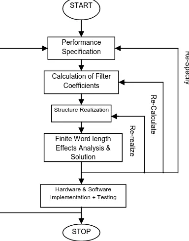
The Digital filters have various stages in their design. The flow chart for the Design of Digital filter is shown in figure 1. An important taskfor the designer is to find values of aiand bi
[image:2.595.86.278.227.472.2]such that the frequency response of the filter approximates a desired characteristic while preserving the stability of the designed filter.
Fig 1: Flow chart of Digital filter design
During design of digital filters, it is important to fulfill accepted design specifications such as: the width of pass-band, width of stop-pass-band, value of pass-band ripples and value of stop-band ripples. Hence, the design of this filter can be considered as an optimization problem of cost function J(w) stated as:
min J(w)
where w=[ a0, a1, a2, …., aL, b1, b2, ….., bM ] is
filter coefficient vector. The aim is to minimize the cost function J(w) by adjusting w. The cost function is usually expressed as the time-averaged cost function defined by:
2
1
(
)
(
)
1
)
(
N
k
d
k
y
k
N
w
J
(3)where d(k) and y(k) are the desired and actual responses of the filter, respectively and N is the number of samples used for the calculation of cost function.
3.
SIMULATED ANNEALING FOR IIR
Simulated Annealing (SA) is a well-known powerful global optimization algorithm, introduced in combinatorial optimizations .It is based on random moves, and has the ability to overcome local minima, found on the way toward a better minimum, with uphill moves. The synthesis of a digital filter transfer function requires that the values of the
multiplier coefficients in the filter implementation be selected such that the transfer function of the filter meets the prescribed frequency response specification. The filter Coefficients are selected in such a way as to minimize the difference between the desired and the actual response. The design process seeks to minimize this "difference" function, known as the objective or cost function. Since the number of filter coefficients can be large, the number of configurations that the filter system can assume becomes very large. An exhaustive search for a coefficient set that minimizes the objective function can only be attempted at great computational expense. To minimize the computational effort, limited systematic or random search methods are relied upon. Simulated annealing is a stochastic optimization technique that has been used for large-scale, discrete space problems. The simulated annealing algorithm, which is based on the theory of statistical mechanics is, essentially an iterative random search procedure with adaptive moves along the coordinate directions. The Metropolis algorithm, which has been widely used in simulated annealing, was originally developed for use in the simulation of a collection of atoms in thermal equilibrium at a given temperature. At each step of this algorithm, an atom is given a small random displacement and the resulting change in the energy of the system (∆E) is computed. The method of simulated annealing consists of three functional relationships.
1. g(x): Probability density of state-space of D parameters x=xi ; {i =1, D}.
2. h(∆E): Probability for acceptance of new cost-function given the just previous value.
3. T(k): schedule of “annealing” the “temperature” T in annealing-time steps k, i.e., of changing the volatility or fluctuations of one or both of the two previous probability densities. The new displacement is accepted subject to the criterion: If ∆E≤ 0, the acceptance probability is based on the chances of obtaining a new state with “energy” Ek+1 relative to a previous state with “energy” ) / exp ( ) / exp ( 1 1 ) / exp ( ) / exp ( ) / exp ( ) ( 1 T E T E T E T E T E E h k k (4)
where ∆E represents the “energy” difference between the present and previous values of the energies (considered here as cost functions) appropriate to the physical problem, i.e., ∆E = Ek1 Ek. This essentially is the Boltzmann distribution contributing to the statistical mechanical partition function of the system. Uniform random deviates in the interval (0, l) are a convenient means of implementing the random part h (∆E). The accepted rearrangement is then used as the starting point of the next step. By repeating the step many times, the algorithm simulates the thermal motion of atoms in thermal contact with a heat bath at temperature T. At very high values of temperature T, in the above expressions, virtually any rearrangement will be accepted. As the temperature falls to low values, rearrangements that increase the change in energy will "re likely be rejected. This strategy allows for controlled "uphill" excursions to be taken and hence to seek "hidden" arrangements with lower energy levels. Using the Metropolis algorithm, simulated annealing has been used for discrete optimization problems. Although the algorithm does not guarantee to find the global optimum, if the function has many good near optimal solutions it will find one. The simulated annealing design process consists of first "melting"
START
Performance Specification
Calculation of Filter Coefficients
Structure Realization
Finite Word length Effects Analysis &
Solution
Hardware & Software Implementation + Testing
the system being optimized at a high temperature and then lowering the temperature in slow stages until the system is "cold", that is until no further changes occur. As in statistical mechanics, the simulation must proceed long enough for the system to attain a steady state at each temperature. An annealing schedule is the sequence of temperatures and rearrangements of the coefficient values attempted to reach steady state at each temperature. An important feature of simulated annealing is that the "gross" features of the function appear at high values of temperature and the "finer" detail at lower values. The aim is to minimize the cost function J(w) as given in eq. 3 by adjusting w. The fitness value of a solution i in the population is determined by using fitness formula given as:
i
w
J
k
i
fit
)
(
1
)
(
(5)where J(w) is the cost function value computed for i and k is the number of poles outside the unit circle.
The summarized pseudo code of SA is shown in figure 2. In the proposed SA, various parameters fixed for analysis have been shown in table 1.
Procedure SA Initialization;
while condition not met new_model=random
delta_E=E(new_model) – E(current_model)
if (delta_E<0) current_model=new_model
else probability P=exp^ (-delta_E /alpha_T) : currnt_model = new_model
[image:3.595.320.522.80.700.2]end while end procedure
[image:3.595.325.522.117.283.2]Fig 2: Pseudo code of Simulated Annealing
Table 1. Parameters for SA Technique
Quantity Values
Temperature Gradient 100
Initial Temperature 100
Temperature update Exponential temperature update Annealing Function Fast Annealing
Function tolerance exp-6
Finishing Condition 100*5
4.
RESULTS AND DISCUSSION
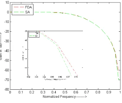
Experiments are carried for well known IIR digital filters (see Appendix), which has been used by many authors as a “benchmark filter” for comparison purpose. To compare the performance of proposed method, the results of fda (filter design analysis) method is also obtained through simulations. The examples were performed on with Pentium IV, 2.80 GHz CPU and 1GB of RAM. Simulation study is carried out in MATLAB to demonstrate the potentiality of SA for the design of IIR digital filters. The magnitude and phase response of first example is shown in figure 3 and figure 4 in which a zoomed in curve for transition band is included. It is observed from the magnitude responses that the gain is -62.61 at 0.9868 using fda, but using proposed method, this gain occurs at 0.9746. This gives us better transition band compared to other technique. It is clear from phase response that phase is identical to fda tool response. In figure 5, we have summarized Pole-Zero behavior of Low pass filter. It can be
seen that the poles-zeros location of designed filter falls with in unit circle. This shows that the designed filter is also stable with proposed method.
Fig 3: Magnitude Response of low pass filter
0 0.1 0.2 0.3 0.4 0.5 0.6 0.7 0.8 0.9 -3
-2.5 -2 -1.5 -1 -0.5 0
Normalized Frequency--->
P
h
a
s
e
i
n
r
a
d
ia
n
--->
[image:3.595.53.282.316.427.2]FDA SA
Fig 4: Phase Response of low pass filter
-1 -0.5 0 0.5 1 -1
-0.8 -0.6 -0.4 -0.2 0 0.2 0.4 0.6 0.8 1
Real Part
Im
a
g
in
a
ry
P
lo
t
Pole-Zero Plot in SA
Fig 5: Pole-Zero plot of low pass filter
[image:3.595.322.523.356.665.2] [image:3.595.49.289.457.559.2]Table 2. Coefficients of Low-pass filter Designed with 2nd order
Table 3 provides a comparison of coefficients of high-pass filter with the filter design tool. On comparison, it is found that the proposed algorithm gives optimal coefficients for High pass filter and least mean square error. It is seen that the optimal coefficients provides minimum value of MSE equal to 2.9963 as compared to 3.0589 using fda.
Table 3. Coefficients of High-pass filter Designed with 3rd order
Coefficients fda tool SA based
a0 0.0004218886 0.0004218886
a1 -0.001687554 -0.00161024
a2 0.0025313316 0.00229933
a3 -0.001687554 -0.0014555
a4 0.0004218886 0.000344561
b1 1 1
b2 3.177811 3.15992
b3 3.8546544 3.80985
b4 2.10730622 2.069939
b5 0.43700264 0.426703
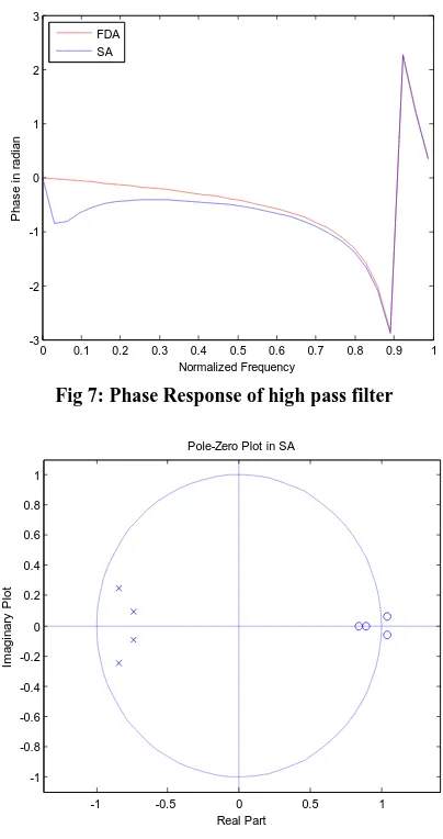
The figure 6 and figure 7 illustrates the magnitude and phase response of second example.Figure 8 summarized Pole-Zero position of High pass filter using SA. It is clearly seen that the poles and zeros placement gives us stable high pass filter.
0 0.1 0.2 0.3 0.4 0.5 0.6 0.7 0.8 0.9 1 -250
-200 -150 -100 -50 0 50
Normalized Frequency
G
a
in
i
n
d
B
[image:4.595.329.528.93.262.2]FDA SA
Fig 6: Magnitude Response of high pass filter
0 0.1 0.2 0.3 0.4 0.5 0.6 0.7 0.8 0.9 1 -3
-2 -1 0 1 2 3
Normalized Frequency
P
h
a
s
e
i
n
r
a
d
ia
n
FDA SA
Fig 7: Phase Response of high pass filter
-1 -0.5 0 0.5 1 -1
-0.8 -0.6 -0.4 -0.2 0 0.2 0.4 0.6 0.8 1
Real Part
Im
a
g
in
a
ry
P
lo
t
Pole-Zero Plot in SA
Fig 8: Pole-Zero plot of high pass filter
5.
CONCLUSION
Optimal IIR digital filter coefficients have been calculated using simulated annealing. The algorithm obtains IIR filter coefficients to approximate a desired magnitude frequency response. The coefficients has been developed which are based on specifications. The values of these specifications are selected after in depth study, expert choice and literature. The Plots of Frequency Response and Pole-Zero of low pass filter and high pass filter is introduced. The Pole-Zero plots discusses the stability of IIR digital filters. The performance of proposed method was compared with fda tool. It is also observed that MSE of low-pass and high pass filter is 0.3284 and 0.29963 respectively, which is least observed as compared to fda technique. The simulation results show that SA has better, or at least equivalent, global search ability but computation time is quite long. The analysis will help the designers/ engineers to decide about the selecting coefficients to attenuate the signal. Further, the other Evolutionary algorithm can be discussed for the design of IIR filters.
6.
APPENDIX
Example 1: In the first example, design a low-pass filter with
following specifications: Pass/Stop band ripples 1dB/ 15dB, and band edges 200Hz / 400Hz and a sampling frequency of 1000Hz.Coefficients fda tool
SA based
a0 0.3752 0.3749
a1 0.7504 0.7489
a2 0.3752 0.3749
b1 1 1
b2 0.3120 0.3109
[image:4.595.65.280.94.197.2] [image:4.595.63.271.522.697.2]Example 2: This example is taken for design of a high-pass filter with following specifications: Pass/Stop band ripples 1dB/ 75dB, and band edges 600Hz / 200Hz and a sampling frequency of 1500Hz.
7.
REFERENCES
[1] Proakis, J. G. and Manolakis, D. G. 2007. Digital Signal Processing: Principles, Algorithms, and Applications. Pearson Education Ltd.
[2] Skaf, Joelle. and Stephen, P. Boyd. 2008. Filter Design with Low Complexity Coefficients. IEEE Transactions on Signal processing. 56(July 2008), 3162-3170.
[3] Vaccaro, Richard J. and Harrison, Brian F. 1996. Optimal Matrix-Filter Design. IEEE Transactions on Signal processing. 44(March 1996), 705-710.
[4] Zhang, Xi. and Iwakura, Hiroshi. 1996. Design of IIR Digital Filters based on Eigen value Problem. IEEE Transactions on Signal processing. 44(June 1996), 1325-1319.
[5] Argenti, Fabrizio. and Enrico, Del Re. 1998. Design of IIR Eigen filters in the Frequency domain. IEEE Transactions on Signal processing. 46(June 1998), 1694-1700.
[6] Yao, Xin., Liu, Yong. and Lin, Guangming. 1999. Evolutionary Programming Made Faster. IEEE Transaction on Evolutionary Computation. 3(July 1999), pp. 83-102.
[7] Chauhan, R.S. and Kamboj, A. 2007. MATLAB based Design of Digital FIR filter using window technique. In Proceeding of IEEE Conf. on Art. Int. Systems.
[8] Kacelenga, R.V. , Graumann, P.V., and Turner, L.E. 1990. Design of filters using simulated annealing. In IEEE Proc. Int. Symp. on Circuits and Systems.
[9] Benvenuto, N. and Marchesi, M. 1992. Applications of simulated annealing for the design of digital filters. IEEE Transaction Signal Processing. 40(Feb. 1992), 323-331.
[10] Abdesselam, K.D. 2000. Design of Stable, causal, perfect reconstruction, IIR Uniform DFT Filters. IEEE
Transactions on Signal processing. 48(April 2000), 1110-1117.
[11] Tseng, C.C. and Pei, S.C. 2001. Stable IIR Notch Filter design with optimal pole placement. IEEE Transactions on Signal processing. 49(Nov. 2001), 2673-2681.
[12] Cousseau, J.E. , Werner, Stefan. and Donate, P.D. 2007. Factorized All-Pass Based IIR Adaptive Notch Filters. IEEE Transaction on Signal Processing. 55(2007), 5225-5236, 2007.
[13] Oliveira, H.A., Petraglia, Antonio. and Petraglia, M.R. 2007. Frequency Domain FIR Filter Design Using Fuzzy Adaptive Simulated Annealing. In IEEE International Symposium on Signal Processing and Information Technology.
[14] Jung, B.W., Yang, H.J. and Chun, J. 2008. Finite Word length Digital Filter Design Using Simulated Annealing. IEEE Transaction Signal Processing, 1(2008), 546-550.
[15] Chauhan, R.S. and Arya, Sandeep K. 2010. Design of IIR digital filter using analog to digital mapping. Journal of Neural Computing Systems. 3(Jan. 2010), 51-55.
[16] Yang, Qi. Ji. 2010. Application of Improved Simulated Annealing Algorithm in Facility Layout Design. In Proceedings of the 29th Chinese Control Conference.
[17] Smith, Kevin I., Everson, Richard M., Fieldsend, Jonathan E., Chris, Murphy. and Misra, Rashmi. 2008. Dominance-Based Multiobjective Simulated Annealing. IEEE Transaction on Evolutionary Computation. 12(June 2008), 323-343.
[18] Ahn, Soyeon., Heedeok, Lee. and Byungwook, Jung. 2011. Medium PRF set selection for pulsed Doppler radars using simulated annealing. IEEE. 1(2011), 90-95.