Performance Evaluation of CMN for Mel-LPC based
Speech Recognition in Different Noisy Environments
Md. Mahfuzur Rahman
Department of Computer Science and Engineering, Comilla University, Comilla,
Bangladesh
Sanjit Kumar Saha
Department of Computer Science and Engineering,
Comilla University, Comilla, Bangladesh
Md. Zakir Hossain
Department of Computer Science and Engineering,
Comilla University, Comilla, Bangladesh
Md. Babul Islam
Department of Applied Physics and Electronic
Engineering, Rajshahi University, Rajshahi, Bangladesh
ABSTRACT
This study is intended to develop a noise robust distributed speech recognizer for real-world applications by employing Cepstral Mean Normalization (CMN) for robust feature extraction. The main focus of the work is to cope with different noisy environments. To realize this objective, Mel-LP based speech analysis has been used in speech coding on the linear frequency scale by applying a first-order all-pass filter instead of a unit delay. Mismatch between training and test phases is reduced through robust feature extraction by applying CMN on Mel-LP cepstral coefficients as an effort to reduce additive noise and channel distortion. The performance of the proposed system has been evaluated on test set A of Aurora-2 database which is a subset of TIDigits database contaminated by additive noises and channel effects. The experiment is conducted on four different noisy environments and the baseline performance, that is, for Mel-LPC the average word accuracy has found to be 59.05%. By applying the CMN on Mel-LP cepstral coefficients, the performance has been improved to 68.02%. It is found that CMN performs significantly better for different noisy environments.
Keywords
Mel-LPC, bilinear transformation, CMN, Aurora 2 database
1.
INTRODUCTION
The performance of Automatic Speech Recognizers (ASRs) has reached to a satisfactory level under controlled and matched training and recognition conditions. Consequently, speech recognition systems have evolved from laboratory demonstrations to a wide variety of real-life applications, for instance, in telecommunication systems, question and answering systems, robotics, etc., distributed speech recognition (DSR) system is being developed for portable terminals. These applications require such ASRs which can be able to maintain the performance at an acceptable level in a wide variety of emerging environmental situations. However, the performance of DSRs’ severely degrades when there is a mismatch between training and test phases, caused by additive noise and channel effect. Environmental noises as well as channel effects contaminate the speech signal and change the data vectors representing the speech, for instance, reduce the dynamic range, or variance of feature parameters within the frame[1][2]. Consequently, a serious mismatch is occurred between training and recognition conditions, resulting in degradation in recognition accuracy.
Noise robust ASR can be achieved in many ways, such as, enhancement of speech signal either in time domain [3] or in
frequency domain [4][5][6][7][8], enhancement in cepstral
domain [9][10][11], that is, feature parameter compensation, and acoustic model compensation or model adaptation[12][13][14]. In HMM based recognizer, the model adaptation approaches have been shown to be very effective to remove the mismatch between training and test environments. However, for a distributed speech recognition system, speech enhancement and parameter compensation approaches are suitable than the model adaptation approach. Because the acoustic model resides at a server, so adaptation or compensation of model from the front-end is not feasible. Therefore, this paper deals with the design of front-end with parameter compensation, such as CMN.
Since the human ear resolves frequencies non-linearly across the speech spectrum, designing a front-end incorporating auditory-like frequency resolution improves recognition accuracy[15][16][17]. In nonparametric spectral analysis, Mel-frequency Cepstral Coefficient (MFCC) [15] is one of the most popular spectral features in ASR. This parameter takes account of the nonlinear frequency resolution like the human speech perception system.
In parametric spectral analysis, the linear prediction coding (LPC) analysis [18][19] based on an all-pole model is widely used because of its computational simplicity and efficiency. While the all-pole model enhances the formant peaks as an auditory perception, other perceptually relevant characteristics are not incorporated into the model unlike MFCC. To alleviate this inconsistency between the LPC and the auditory analysis, several auditory spectra have been simulated before the all-pole modeling
[16][[20][21][22]
.
In contrast to the different spectral modification, Strube [23]
proposed an all-pole modeling to a frequency warped signal which is mapped onto a warped frequency scale by means of the bilinear transformation [24], and investigated several computational procedures. However, the methods proposed by Oppenheim and Johnson [24] to estimate warped all-pole model have rarely been used in automatic speech recognition. Recently, as an LP-based front-end, a simple and efficient time domain technique to estimate all-pole model is proposed by Matsumoto et al.[25], which is referred to as a “Mel-LPC” analysis. In this method, the all-pole model has been estimated directly from the input signal without applying bilinear transformation. Hence, the prediction coefficients can be estimated without any approximation by minimizing the prediction error power at a two-fold computational cost over the standard LPC analysis.
2.
MEL-L P ANAL YSI S
The frequency-warped signal
~
x
[
n
]
(
n
0
,
,
)
obtained by the bilinear transformation [24] of a finite length windowed signalx
[
n
]
(
n
0
,
1
,
,
N
1
)
is defined by
1 0 0]
[
)
(
~
]
[
~
)
~
(
~
N n n n nz
n
x
z
X
z
n
x
z
X
(1)where
~
z
1 is the first-order all-pass filter,1 1 1
.
1
~
z
z
z
(2)where
0
1
is treated as frequency warping factor.The phase response of
~
z
1 is given by
cos
1
sin
tan
2
~
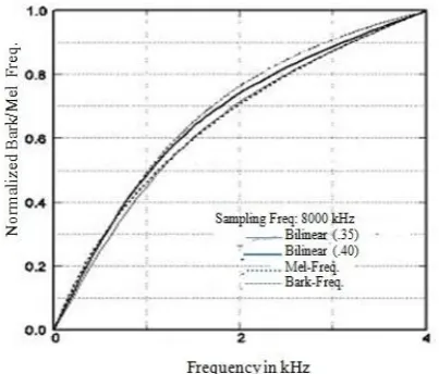
1 (3) [image:2.595.62.264.381.553.2]This phase function determines a frequency mapping. As shown in Fig. 1,
0
.
35
and
0
.
40
can approximate the mel-scale and bark-scale [26][27] at the sampling frequency of 8 kHz respectively.Fig. 1: The frequency mapping functions by bilinear transformation.
Now, the all-pole model on the warped frequency scale is defined as
p k k k ez
a
z
H
1~
~
1
~
~
~
(4)where
a
~
k is the k-th mel-prediction coefficient and
~
e2 is the residual energy[23].On the basis of minimum prediction error energy for
~
x
[
n
]
over the infinite time span,
a
~
k and
~
e are obtained by Durbin’s algorithm from the autocorrelation coefficients]
[
~
m
r
of~
x
[
n
]
defined by
0]
[
~
]
[
~
]
[
~
nm
n
x
n
x
m
r
(5)which is referred to as mel-autocorrelation function.
The mel-autocorrelation coefficients can easily be calculated from the input speech signal
x
[
n
]
via the following two steps[25][28]
. First, the generalized autocorrelation coefficients are calculated as
1 0]
[
]
[
]
[
~
N n mn
x
n
x
m
r
(6)where
x
m[
n
]
is the output signal of an m-th order all passfilter
z
~
m excited byx
0[
n
]
x
[
n
]
. That is,~
r
[
m
]
isdefined by replacing the unit delay
z
1 with the first order all-pass filter~
z
(
z
)
1 in the definition of conventional autocorrelation function as shown in Fig. 2.Fig. 2: Generalized autocorrelation function.
Due to the frequency warping,
~
r
[
m
]
includes the frequency weighting ~( )~
j
e
W defined by
1 2
~
1
1
)
~
(
~
z
z
W
(7)which is derived from
2 ~
)
(
~
~
je
W
d
d
(8)Thus, in the second step, the weighting is removed by inverse filtering in the autocorrelation domain using
1
1)
~
(
~
)
~
(
~
z
W
z
W
.As feature parameters for recognition, the Mel-LP cepstral coefficients can be expressed as:
0~
)
~
(
~
log
n n kz
c
z
(9)where
c
k
are the mel-cepstral coefficients.The mel-cepstral coefficients can also be calculated directly from mel-prediction coefficients
a
~
k [29]using the following recursion:
1 1~
)
(
1
~
k j j k k kk
k
j
a
c
k
a
c
(10)It should be noted that the number of cepstral coefficients need not be the same as the number of prediction coefficients.
Cross
Corr.
mz
z
~
.
]
[
n
x
m]
[
n
3.
ENHANCEMENT
OF
MEL-LP
CEPSTRUM
3.1
Ceps tral Mean Normali zation
A robust speech recognition system must adapt with its acoustical environment or channel. To bring this concept in effect, a number of normalization methods have been developed in the cepstral domain so far. The simplest but effective cepstral normalization method is the Cepstral Mean Normalization (CMN) technique [9]. In CMN, the mean of the cepstral vectors over an utterance is subtracted from the cepstral coefficients in each frame as given below:
Nn
m
c
n
N
n
c
n
c
0
]
[
1
]
[
]
[
(11)where
c
[
n
]
andc
m[
n
]
are the time-varying cepstral vectors of the utterance before and after CMN, respectively, and N is the total number of frames in the utterance.The average of the cepstrum vectors over the speech interval represents the channel distortion, which does not use any knowledge of the environment [10]. As the channel distortion is suppressed by CMN, it can be viewed as parameter filtering operation. Consequently, CMN has been treated as high-pass and band-pass filters [11]. The effectiveness of CMN for the combined effect of additive noise and channel distortion is limited. Acero and Stern [30] have developed more complex cepstral normalization techniques to compensate the joint effect of additive noise and channel distortion.
4.
EVAL UAT ION ON AURO RA 2
DAT ABASE
4.1
Experi men tal Setup
The proposed system was evaluated on Aurora-2 database [31],
which is a subset of TIDigits database [32] contaminated by additive noises and channel effects. This database contains the recordings of male and female American adults speaking isolated digits and sequences up to 7 digits. In this database, the original 20 kHz data have been down sampled to 8 kHz with an ideal low-pass filter extracting the spectrum between 0 and 4 kHz. These data are considered as clean data. Noises are artificially added with SNR ranges from 20 to -5 dB at an interval of 5 dB.
To consider the realistic frequency characteristics of terminals and equipment in the telecommunication area an additional filtering is applied to the database. Two standard frequency characteristics G.712 and MIRS are used which have been defined by ITU [33].
[image:3.595.313.540.235.350.2]It should be noted that the whole Aurora 2 database was not used in this experiment rather a subset of this database was used as shown in Table 1.
Table 1: Definition of training and test data
The recognition experiments were conducted with a 12th order prediction model of Mel-LPC analysis. The pre-emphasized speech signal with a pre-emphasis factor of 0.95 was windowed using Hamming window of length 20 ms with 10 ms frame period. The frequency warping factor was set to
0.35. As front-end, 14 cepstral coefficients and their delta coefficients including 0th terms were used. Thus, each feature vector size is 28.
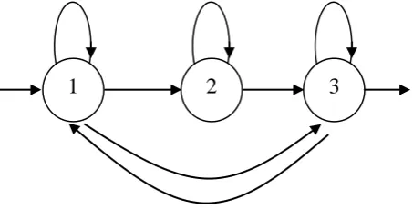
The reference recognizer was based on HTK (Hidden Markov Model Toolkit, version 3.4) software package. The HMM was trained on clean condition. The digits are modeled as whole word HMMs with 16 states per word and a mixture of 3 Gaussians per state using left-to-right models. In addition, two pause models ‘sil’ and ‘sp’ are defined. The ‘sil’ model consists of 3 states which illustrates in Fig. 3. This HMM shall model the pauses before and after the utterance. A mixture of 6 Gaussians models each state. The second pause model ‘sp’ is used to model pauses between words. It consists of a single state, which is tied with the middle state of the ‘sil’ model.
Fig. 3: Possible transition in the 3-state pause model ‘sil’.
The recognition accuracy (Acc) is evaluated as follows:
%
100
N
I
S
D
N
Acc
(12)
where N is the total number of words. D, S and I are deletion, substitution and insertion errors, respectively.
4.2
Experimental Results
The detail recognition results are presented in this section. The word accuracy for Mel-LPC without applying CMN is listed in Table 2 which is considered as baseline result. The average word accuracy over all noises within the set A and over SNRs 20 to 0 dB is found to be 59.05% for the baseline. The word accuracy with CMN is given in Table 3. The average recognition performance of Mel-LPC with CMN is found to be 68.03%.
Performance of CMN on different noise types is demonstrated in Fig.4. It is also observed that the larger improvements are achieved for babble and car noises with CMN as compared to baseline performance. The average recognition accuracy does not differ significantly for subway and exhibition noises. Effect of CMN found from the study on different noise levels is demonstrated in Fig.5. It is observed that greater improvements in recognition accuracy are achieved for 15 dB to 0 dB speech signals. It has also been noticeable that, whatever might be the noise levels, the recognition accuracy doesn’t improve significantly for subway and exhibition noises.
5.
CONCLUSION
An HMM-based automatic speech recognizer (ASR) was developed and as an enhancement technique in the cepstral domain, the performance of CMN on Mel-LPC was evaluated on test set A of Aurora 2 database. It is observed that the CMN has significant effect for babble and car noises. It is also found that CMN exhibits best performance for babble noise. The average word accuracy does not differ significantly for subway and exhibition noises after applying CMN. The Filter Data
set
Noise Type SNR [dB]
Training G.712 Clean ∞
Test G.712
Test set A
Subway, babble, car, exhibition
clean, 20, 15, 10, 5, 0, -5
3
2
recognition performance for babble and car noises has been improved from 48.06% to 70.90% and from 53.77% to 66.49% respectively. The overall recognition accuracy has been improved from 59.05% to 68.03%. The improvement is also significant for 15 dB to 0 dB speech signals.
No significant improvement has been found for any level of subway and exhibition noises present in the speech signal.
[image:4.595.46.558.108.756.2]Table 2: Word accuracy [%] for MLPC without CMN (baseline).
Table 3: Word accuracy [%] for MLPC with CMN.
Fig.4: Performance of CMN for Different Noisy Environments
Fig.5: Effect of CMN on different noise levels.
30 40 50 60 70
Subway Babble Car Exhibition
A
cc
u
rac
y
(%
)
Noise Types
Effect of CMN on Different Noisy Environments
With CMN
Without CMN
0 20 40 60 80 100
cln 20dB 15dB 10dB 5dB 0dB -5dB
A
cc
u
rac
y
(%
)
Noise Levels in SNR[dB]
Performance of CMN on Different Levels of Noisy
Environments
With CMN
Without CMN
Noise SNR [dB] Average
(20 to 0 dB)
clean 20 15 10 5 0 -5
Subway 98.71 96.93 93.43 78.78 49.55 22.81 11.08 68.30
Babble 98.61 89.96 73.76 47.82 21.95 6.80 4.44 48.06
Car 98.54 95.26 83.03 54.25 24.04 12.23 8.77 53.77
Exhibition 98.89 96.39 92.72 76.58 44.65 19.90 11.94 66.05
Average 98.69 94.64 85.74 64.36 35.05 15.44 9.06 59.05
Noise SNR [dB] Average
(20 to 0 dB)
clean 20 15 10 5 0 -5
Subway 99.02 96.41 92.05 78.66 50.23 24.78 16.09 68.43
Babble 98.82 97.37 93.80 82.22 55.32 25.76 13.30 70.90
Car 98.87 96.96 92.72 77.42 42.77 22.55 13.18 66.49
Exhibition 99.07 96.08 91.67 76.70 45.97 20.98 11.60 66.28
6.
REFERENCES
[1] Bateman, D. C., et al., 1992. Spectral contrast normalization and other techniques for speech recognition in noise. Proc. of ICASSP ’92, I: 241-244.
[2] Vaseghi, S. V. and B.P. Milner, 1993. Noise-adaptive hidden Markov models based on Wiener filters. Proc. of Eurospeech ’93, II: 1023-1026.
[3] Islam, M. B., K. Yamamoto, H. Matsumoto, 2007. Mel-Wiener filter for Mel-LPC based speech recognition. IEICE Transactions on Information and Systems, E90-D (6): 935-942.
[4] Boll, S. F., 1979. Suppression of acoustic noise in speech using spectral subtraction. IEEE Trans. Acoust., Speech and Signal Processing, 27(2): 113-120.
[5] Lim, J. S. and A.V. Oppenheim, 1979. Enhancement and bandwidth compression of noisy speech. Proc. of the IEEE, 67(2): 1586-1604.
[6] Lockwood, P. and J. Boudy, 1992. Experiments with a nonlinear spectral subtractor (nss), hidden Markov models and the projection or robust speech recognition in cars. Speech Commun., 11(2-3): 215-228.
[7] Agarwal, A. and Y. M. Cheng, 1999. Two-stage Mel-warped Wiener filter for robust speech recognition. Proc. of ASRU ’99: 67-70.
[8] Zhu, Q. and A. Alwan, 2002. The effect of additive noise on speech amplitude spectra: A Quantitative analysis. IEEE Signal Processing Letters, 9(9): 275-277.
[9] Atal, B., 1974. Effectiveness of linear prediction characteristics of the speech wave for automatic speaker identification and verification. J. Acoust. Soc. Am. 55(6): 1304-1312.
[10]Furui, S., 1981. Cepstral analysis technique for automatic speaker verification. IEEE Trans. Acoust., Speech and Signal Processing, ASSP-29: 254-272.
[11]Mokbel, C., et al., 1984. Compensation of telephone line effects for robust speech recognition. Proc. of ICSLP ’94: 987-990.
[12]Gales, M. J. F. and S. J. Young, 1993a. HMM recognition in noise using parallel model combination. Proc. of Eurospeech ’93, II: 837-840.
[13]Gales, M. J. F. and S. J. Young, 1993b. Cepstral parameter compensation for HMM recognition in noise. Speech Communication, 12(3): 231-239.
[14]Varga, A. P. and R. K. Moore, 1990. Hidden Markov model decomposition of speech and noise. Proc. of ICASSP ’90, 2: 845-848.
[15]Davis, S. and P. Mermelstein, 1980. Comparison of parametric representations for monosyllabic word recognition in continuously spoken sentences. IEEE Trans. on Acoustics, Speech, and Signal Processing, ASSP-28(4): 357-366.
[16]Hermansky, H., 1987. Perceptual linear predictive (PLP) analysis of speech. J. Acoust. Soc. Am., 87(4): 17-29.
[17]Virag, N., 1995. Speech enhancement based on masking properties of the auditory system. Proc. ICASSP ’95: 796-799.
[18]Itakura, F. and S. Saito, 1968. Analysis synthesis telephony based upon the maximum likelihood method. Proc. of 6th International Congress on Acoustics, Tokyo: C-5-5, C17-20.
[19]Atal, B. and M. Schroeder, 1968. Predictive coding of speech signals. Proc. of 6th International Congress on Acoustics, Tokyo: 21-28.
[20]Makhoul, J. and L. Cosell, 1976. LPCW: An LPC vocoder with linear predictive warping. Proc. of ICASSP ’76: 446-469.
[21]Itahashi, S. and S. Yokoyama, 1987. A formant extraction method utilizing mel scale and equal loudness contour. Speech Transmission Lab.-Quarterly Progress and Status Report (Stockholm) (4): 17-29.
[22]Rahim, M. G. and B. H. Juang, 1996. Signal bias removal by maximum likelihood estimation for robust telephone speech recognition. IEEE Trans. on Speech and Audio Processing, 4(1): 19-30.
[23]Strube, H. W., 1980. Linear prediction on a warped frequency scale. J. Acoust. Soc. Am., 68(4): 1071-1076.
[24]Oppenheim, A. V. and D. H. Johnson, 1972. Discrete representation of signals. IEEE Proc., 60(6): 681-691.
[25]Matsumoto, H., et al., 1998. An efficient Mel-LPC analysis method for speech recognition”, Proc. ICSLP ’98: 1051-1054.
[26]Zwicker, E. and E. Terhardt, 1980. Analytical expressions for critical band rate and critical bandwidth as a function. J. Acoust. Soc. Am., 68: 1523-1525.
[27]Lindsay, P. H. and D. A. Norman, 1977. Human information processing: An introduction to psychology. 2nd Edn., Academic Press.
[28]Nakagawa, S., et al., ed., 2005. Spoken language systems. Ohmsha, Ltd., Japan, ch.7.
[29]Markel, J. and A. Gray, 1976. Linear prediction of speech. Springer-Verlag.
[30]Acero, A. and R. Stern, 1990. Environmental robustness in automatic speech recognition. Proc. of ICASSP ’90: 849-852.
[31]Hirsch, H. G. and D. Pearce, 2000. The AURORA experimental framework for the performance evaluation of speech recognition systems under noisy conditions. Proc. ISCA ITRW ASR 2000: 181:188.
[32]Leonard, R. G., 1984. A database for speaker independent digit recognition. ICASSP84, 3: 42.11.
![Table 3: Word accuracy [%] for MLPC with CMN.](https://thumb-us.123doks.com/thumbv2/123dok_us/8097288.786562/4.595.46.558.108.756/table-word-accuracy-mlpc-cmn.webp)
