An Optimal Fast Full Search Motion Estimation and
Suboptimal Motion Estimation Algorithms
Adapa Venkata Paramkusam
Electronics and Communication WISTM Engineering College AU, Visakhapatnam, Andhra Pradesh, India
V.S.K. Reddy
Member, IEEE
Electronics and Communication M.R. College of Engineering & Technology JNTUH, Hyderabad, Andhra Pradesh, India
ABSTRACT
The new fast full search motion estimation algorithm for optimal motion estimation is proposed in this paper. The Fast Computing Method (FCM) which calculates the tighter boundaries faster by exploiting the computational redundancy and the Best Initial Matching Error Predictive Method (BIMEPM) which predicts the best initial matching error that enables the early rejection of highly impossible candidate blocks are presented in this paper. The proposed algorithm provides the optimal solution with fewer computations by utilizing these two methods FCM and BIMEPM. Experimental results show that the proposed new fast full search motion estimation algorithm performs better than other previous optimal motion estimation algorithms such as Successive Elimination Algorithm (SEA), Multilevel Successive Elimination Algorithm (MSEA) and Fine Granularity Successive Elimination (FGSE) on several video sequences. The operation number for this proposed algorithm is reduced down to 1/52 of Full Search (FS). But MSEA and FGSE algorithms can reduce computations by 1/40 and 1/42 of FS. Finally, the proposed new fast full search motion estimation algorithm is modified to sub optimal motion estimation algorithm introducing only a small average PSNR drop of around 0.2dB but achieves very fast computational speed. The superior performance of this sub optimal motion estimation algorithm over some fast motion estimation algorithms is also proved experimentally.
General Terms
Video coding, video processing.
Keywords
Successive elimination algorithm; fast full search; motion estimation; motion vector; suboptimal motion estimation.
1.
INTRODUCTION
The main objective of Block-matching algorithm for motion estimation is to find the best matched candidate block in the reference frame for every macroblock in the current frame, according to a predetermined matching error criterion. The displacement between these two blocks defines a motion vector. Some of the matching errors used are Sum of Absolute Difference (SAD), Sum of Squared Difference (SSD) and the Cross Correlation Function (CCF). In most situations the SAD is used as matching error because it does not require any multiplication and gives similar performance as the mean square error. The full search block matching algorithm examines all the (2W+1)2 candidate blocks in the search window to find the best-matched candidate block that produces the minimum matching error with a maximum displacement of W pixels/frame. To reduce the computational load of full search, many fast search algorithms such as Three
step search algorithm(3SS)[1], new three-step search algorithm(N3SS)[2], diamond search algorithm(DS)[3], hexagon-based search algorithm (HEXBS)[4], and Unsymmetrical-cross Multi-Hexagon-grid Search (UMHexagonS) [5][6] have been proposed. These algorithms use pre defined search patterns to reduce the search points in the search window. If the actual motion is not matched with the search pattern then the both speed and quality will decrease. Moreover these algorithms are easily trapped to local minimum and hence sub optimal motion vectors are obtained. For the optimal solution with reduced computations, Successive elimination algorithm [7] or modified versions based on SEA [8, 9] are preferred. These algorithms provide the optimal solution as that of full search, but with less operation number by eliminating highly impossible candidate blocks as early as possible to reduce the computational cost. In this paper, we propose both optimal and sub optimal solutions for block motion estimation based on best initial matching error predictive method. The proposed new fast full search motion estimation provides optimal solution by utilizing Fast Computing Method (FCM) and Best Initial Matching Error Predictive Methods (BIMEPM). The new fast full search motion estimation is slightly modified to reduce the computational load further but relaxes optimality. The rest of this paper is organized as follows. Some well-known fast full-search algorithms are reviewed In Section 2. Then, we present the new fast full search motion estimation algorithm and its modified versions which utilize FCM and BIMEPM methods in section 3. In Section 4, the simulation results for the proposed and the conventional methods are compared to verify the performance of the proposed algorithms. Finally, conclusions are given in Section 5.
2.
REMARKS ON SEA, MSEA AND
FGSE ALGORITHMS
Successive Elimination Algorithm offers tighter boundaries by partitioning the sum norms in a multilevel manner [8]. First, the block with size of N × N is partitioned into four sub-blocks with a size of N/2 × N/2 and then each sub-block is partitioned into four sub-blocks with a size of N/4 × N/4. This procedure is repeated until the size of the sub-block becomes 2×2. In MSEA, one candidate block is evaluated sequentially from the lowest to the highest level. If the candidate block is eliminated at any level then that candidate block need not be evaluated for the remaining levels. In MSEA, the more non best candidate blocks can be eliminated by tightening the distortion boundaries. FGSE algorithm [9] uses more number of lower boundaries than MSEA to reduce the gap between adjacent boundaries. Thus, FGSE has more chance to eliminate the non best candidates than MSEA before calculating the SAD. It utilizes the boundary value at any level while calculating the boundary at next level thus FGSE algorithm is computationally efficient than MSEA. The main limitations of the SEA, MSEA and FGSE algorithms are: The efficiency of these algorithms depend on initial matching error. If initial matching error is small then more successive tests have a less SADmin and may be skipped. The early rejection of highly impossible candidate blocks depends on the good initial matching error, but there is no method specified in these algorithms to predict better initial minimum SAD. The computational redundancy is not identified between any two adjacent boundaries while computing the boundaries. To fulfill these shortages of these algorithms, a new fast full search motion estimation algorithm is proposed in the following.
3.
PROPOSED ALGORITHM
The proposed new fast full search motion estimation algorithm traces global optimal as traced by the full search but with less computational load. In this proposed algorithm the non best candidate blocks are eliminated by tightening the boundaries but by taking fewer computations to calculate tighter boundaries. This is obtained by using the FCM. The BIMEPM predicts the best initial matching error that enables the early rejection of candidate blocks facilitating to reduce computations. The best initial matching error is predicted basing on the assumption that a good matching candidate block with a small SAD value will also likely to have smaller tighter boundary values. The SAD between between a macro block of size N ×N at position (p, q) in the current frame ft
and the candidate block at position (p + x, q + y) in the reference frame ft-1 is defined as follows
) ( ) , ( ) , ( ) ,
( N 1 1
0 i 1 N 0 j j y q i x p 1 t f j q i p t f y x
SAD
Where x and y are the horizontal and vertical components of the motion vector. According to the inequality |a| + |b| ≥ |a + b|, where a, b ∈ R, the boundary in SEA is derived by performing absolute operation on the difference between sum norms of the macro block and candidate blocks as in eq (2).
) ( ) , ( ) , ( ) , ( 2 1 N 0 i 1 N 0 j 1 N 0 i 1 N 0 j j y q i x p 1 t f j q i p t f y x SEA
A fast algorithm to calculate the sum norms of candidate blocks at every search position is presented in [7]. First, the column sums (sum of pixels in column) are calculated for every possible column of the reference frame. These column sums are calculated quickly by reusing accumulated sum of
overlapped area of vertical adjacent columns. In the second step, the column sums are summed up in a horizontal direction using the same technique to compute the sum norms at every search position in reference frame. Let St (p, q) and
St-1(p, q) represent the sum norms at position (p, q) in the
current frame and reference frames respectively and Ct (p, q)
and Ct-1 (p, q) represent the column sums of columns at (p, q)
in the current frame and reference frames respectively. Then the SEA boundary can be expressed in column sums as
) , ( ) , ( ) , ( ) , ( ) , ( y q x p 1 t S q p t S 1 N 0 i 1 N 0 j 1 N 0 i 1 N 0 j j y q i x p 1 t f j q i p t f y x SEA ) 3 ( 1 0 1 0 ) , ( 1 ) , ( N i N i y q i x p t C q i p t C Where , ) , ( ) , ( , ) , ( ) , ( 1 N 0 i 1 N 0 j j q i p 1 t f q p 1 t S 1 N 0 i 1 N 0 j j q i p t f q p t S 1 N 0 j j q p 1 t f q p 1 t C and 1 N 0 j j q p t f q p t C ) , ( ) , ( ) , ( ) , (
The SEA boundary is treated as first boundary (BV_1) in our proposed algorithm, i.e. BV_1=SEA(x, y). If an absolute operation is performed on the difference not between the sum of column sums, but between column sums, it gives a second boundary value greater than BV_1.
)
(
)
,
(
)
,
(
_
N
1
4
0
i
y
q
i
x
p
1
t
C
q
i
p
t
C
2
BV
The onward boundaries are obtained by replacing the absolute of the difference between each pair of column sums by sum of absolute differences between pixels in that pair of columns.
)
(
)
,
(
)
,
(
)
,
(
)
,
(
_
6
1
N
2
i
y
q
i
x
p
1
t
C
q
i
p
t
C
1
0
i
1
N
0
j
j
y
q
i
x
p
1
t
f
j
q
i
p
t
f
4
BV
………. ) ( ) , ( ) , ( ) , ( ) _( 7 y x SAD 1 N 0 i 1 N 0 j j y q i x p 1 t f j q i p t f 2 N BV There are N+2 boundaries in this proposed algorithm. The last boundary is SAD. These boundaries except first one are computed by FCM proposed in this paper.
3.1
Fast Computing Method (FCM)
Any tighter boundary in this proposed algorithm is obtained by replacing the sum norm difference between two sets of numbers in previous boundary by SAD between these two sets of numbers. The boundaries from BV_2 to BV_N+2 are successively calculated using FCM that is any boundary is updated by using previous boundary. The difference between any two successive boundaries (from BV_3 to BV_ (N+2)) is calculated as follows
)
(
,
)
,
(
)
,
(
)
,
(
)
,
(
)
_(
)
_(
8
1
N
to
0
i
y
q
i
x
p
C
q
i
p
C
1
N
0
j
j
y
q
i
x
p
1
t
f
j
q
i
p
t
f
2
i
BV
3
i
BV
tt
Suppose Ct (p+i, q) - Ct-1 (p+x+i, q+y) > 0 then
)
(
)
,
(
)
(
)
,
(
)
(
)
,
(
)
,
(
)
,
(
)
,
(
)
,
(
)
,
(
)
,
(
)
,
(
9
j
q
i
p
t
f
0
j
D
j
y
q
i
x
p
1
t
f
0
j
D
j
y
q
i
x
p
1
t
f
j
q
i
p
t
f
j
y
q
i
x
p
1
t
f
j
q
1
N
0
j
i
p
t
f
y
q
i
x
p
1
t
C
q
i
p
t
C
y
q
i
x
p
1
t
C
q
i
p
t
C
Where D (j) = ft (p+i, q+j) - ft-1 (p+x+i, q+y+j). Now the
boundaries BV_ (i+3) for i=0 to N-1 can be expressed as follows
) , ( ) ( ) , ( ) ( ) , ( ) , ( ) , ( ) ( ) , ( ) ( ) , ( ) , ( ) ( _ ) _( j q i p t f 0 j D j y q i x p 1 t f 0 j D j y q i x p 1 t f j q i p t f j q i p t f 0 j D j y q i x p 1 t f 0 j D j y q i x p 1 t f j q i p t f 2 i BV 3 i BV ) ( ) , ( ) ( ) , ( ) ( _ 10 j q i p t f 0 j D j y q i x p 1 t f 2 2 i BV
Similarly if Ct (p+i, q) - Ct-1 (p+x+i, q+y) < 0 then it follows
that
)
(
)
,
(
)
(
)
,
(
)
(
_
)
(
_
11
j
y
q
i
x
p
1
t
f
0
j
D
j
q
i
p
t
f
2
i
BV
3
i
BV
If Ct (p+i, q) - Ct-1 (p+x+i, q+y) = 0 then eq (10) or (11) can
be used to find the boundaries. The boundary BV_2 is updated from BV_1 by checking the sign of the block sum norm difference. If St(p, q) > St-1(p, q) then BV_2 can be updated
as follows 0 i M 12 q i p t C y q i x p 1 t C 2 1 BV 2 BV ) ( ) ( ) , ( ) , ( _ _
If St (p, q) < St-1 (p, q) then BV_2 can be calculated as follows
0 i M 13 y q i x p 1 t C q i p t C 2 1 BV 2 BV ) ( ) ( ) , ( ) , ( _ _
Where M (i) = Ct (p+i, q) - Ct-1 (p+x+i, q+y). In conventional
boundary calculation, the operations of subtraction, absolution and addition will take place at each pixel essentially. Whereas in this method initially checking is made of the sign of ft (., .) - ft-1(., .) at each pixel and if the sign is found
boundaries calculation and hence this redundancy can be removed by FCM. Figure 1 shows the %Redundancy per macroblock in a cricket and flower video sequences.
1 50 100 150 200 250
76 78 80 82 84 86 88 90 92 94 96
FRAME NUMBER
%
R
E
D
U
N
D
A
N
C
Y
F l o w e r v i d e o
[image:4.595.57.282.111.272.2]C r i c k e t v i d e o
Figure 1: The percentage of pixels per macroblock (%Redundancy) that do not contribute in the SAD calculation in a cricket and flower videos on frame by
frame basis.
3.2
Refinement phase to pick best initial
motion vector
While comparing the blocks with the tighter boundaries if the initial prediction is good, then more successive tests have a less SADmin and may be skipped. If a block with less SAD is found early while scanning the candidate blocks in a search window, then more candidate blocks can be eliminated in subsequent searches that results in obtaining reduction of computational complexity. In this paper a simple method, BIMEPM is proposed to predict good matching candidate with a small SAD value. This method is based on the assumption that a good matching candidate with a small SAD value will also likely to have smaller lower tighter boundary values. The proposed new fast full search motion estimation algorithm employs two phases. In the first phase, a set of a possible motion vector set (PMV set) is determined. In the second phase, a best motion vector in PMV set is predicted and global minimum point among the search points in the PMV set is determined. The outline of the proposed algorithm is as follows:
First phase:
The motion vector of the corresponding block in the previous frame is selected as an initial motion vector. The SAD at that motion vector is assumed to be SADmin. At each search point of the search window, BV_1 is
calculated initially. If it is less than SADmin, then BV_2is calculated and compared with SADmin. If BV_2is also less than SADmin that checked point is a possible motion vector
and placed in the PMV set. Second phase (BIMEPM):
Find the motion vector with the smallest BV_2 in the PMV set. Calculate the SAD at this motion vector and compare with SADmin. The search position with smallest SAD between these two points is treated as a best initial motion vector.
Now find the global minimum point among the search points in the PMV set by computing the boundaries (BV_2 to BV_ (N+2)) and comparing with up-to-date
SADmin sequentially. While comparison, if the boundary at any stage is greater than SADmin reject that point and
stop the calculation of remaining boundaries
The BIMEPM finds the good matching block in PMV set according to their BV_2 values. So, the good matching block may arrive at starting stage and thereby next subsequent candidate blocks will be obviously eliminated at lower levels of boundary values. If the number of motion vectors in PMV set is equal to zero, then skip second phase (BIMEPM) and the index of the initial motion vector predicted in first phase will be the true motion vector.
3.3
Modified fast motion estimation
algorithm
In this paper the emphasis is also made on suboptimal motion estimation as this process helps to reduce the number of computations without much quality variation in comparison with the optimal motion estimation. Suppose all the points in PMV set are sorted according to their BV_2 values (the points with small BV_2 values appears first) and the global minimum point is found by testing all the points, practically it is observed by exhaustive study on various video sequences that the true motion vector appears in the starting locations of the sorted PMV set. So instead of testing all the points, find the n search points with the smallest BV_2 in the PMV set and compare only among them. As the selective n search points are tested, the number of computations is invariably reduced. The highly impossible candidate blocks are rejected while comparing with boundaries BV_1 and BV_2 causing the search points in PMV to have less possible variation in their SAD values that results insignificant degradation of quality even in the condition that the global minimum point is not found in the selected n search points. In case, the highly impossible candidate blocks are not even rejected while comparing with boundaries BV_1 and BV_2, the quality variation is mostly insignificant because they may be eliminated during the sorting process. The results of modified fast motion estimation algorithm will be the same as FS when the true motion vector is located within n search points. Therefore, larger n improves the video quality while smaller n saves more computation. Generally speaking, the n parameter provides an easy trade off between speed and quality. The experiments have conducted on various video sequences with n values from 1 to 10. Let the number of motion vectors in PMV set is m. In case the m is less than selected n then the best motion vector is found among these m motion vectors.
4.
SIMULATION RESULTS
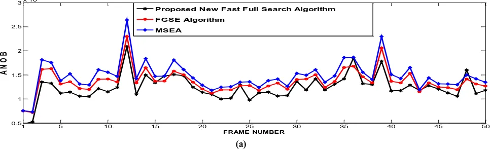
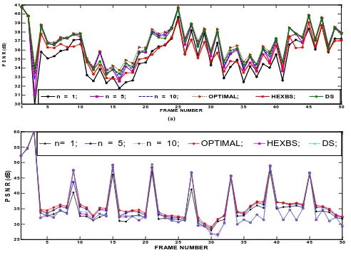
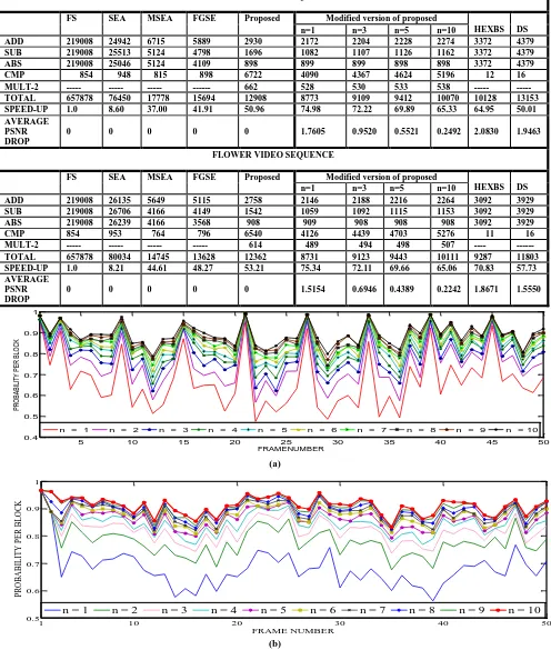
estimation algorithm.The average numbers of total operations per macroblock (ANOB) on frame by frame basis for “cricket” and “flower” video sequences are also shown graphically in the Figure 3 (a) and 3 (b). It is clear from these figures and table that the computational complexity is drastically reduced as compared with FS, SEA, MSEA and FGSE algorithms. The proposed new fast full search motion estimation algorithm is able to achieve a reduction of the computations up to 84% of the SEA, 27% of the MSEA and 15% of the FGSE algorithms. The proposed new fast full search motion estimation algorithm takes fewer computations as compared with MSEA and FGSE algorithm in almost all frames and is shown in the Figure 3 (a) and 3 (b).The modified fast motion estimation algorithm is compared with optimal and well noted suboptimal motion estimation methods Hexagon based search (HEXBS) and Diamond search (DS) using the following two test criteria: Average number operations per macroblock and average peak signal to noise ratio (PSNR). The average numbers of operations per macroblock for various values of n are shown in Table-1. It is clear from this table that even if n is 1 average PSNR drop is less than DS and HEXBS algorithms. The modified fast motion estimation algorithm is able to achieve a further reduction of the computations up to 33% to 16% of the proposed fast full search motion estimation for n values from 1 to 10, introducing only a small quality penalty around 0.2492dB for n=10 and 1.7605dBfor n=1. PSNR (dB) values of modified fast motion estimation algorithm (n =1,5 and 10) are compared with proposed fast full search motion estimation, Hexagon based search and Diamond search algorithms for flower and cricket videos on frame by frame basis are shown in Figure 4 (a) and 4 (b) respectively. From these figures it is observed that modified fast motion estimation algorithm shows better PSNR (dB) values than Hexagon based search and Diamond search algorithms. Since the selective n search positions are tested in PMV set, the probabilities of getting true motion vector for all macro blocks are experimentally studied on different video sequences. Figure 5 (a) and 5 (b) plot probability of getting true motion vector per macroblock in modified fast motion estimation algorithm (n= 1 to 10) for cricket and flower video sequences on frame by frame basis. From these figures, it is observed that the probability of finding global minimum point is about 0.65 and 0.95 when n value is 1 and 10 respectively.
5.
CONCLUSION
The experiments made upon the proposed algorithms new fast full search motion estimation algorithm and modified fast motion estimation algorithm demonstrate that number of computations can be reduced. The former algorithm reduces the required computations to achieve optimal motion vector using two methods. The first method, FCM calculates the tighter boundaries faster by exploiting the computational redundancy. Thus the computational complexity of any algorithm based on MSEA can be reduced by this method. The second one, BIMEPM predicts the best initial matching error that enables the early rejection of candidate blocks facilitating to reduce computations. Experimental results show that the former algorithm can achieve better performance than MSEA and FGSE algorithms. The latter one is the slightly modified one of the former. In this algorithm the computations needed are very less having less quality degradation. This can be achieved by finding out better n value. The study has been made in comparison with the noted Suboptimal Motion Estimation methods like Hexagon based search and Diamond search and proven experimentally comprehensive and qualitative.
1 5 10 15 20 25 30 35 40 45 50
0.5 1 1.5 2 2.5
3x 10
4
FRAME NUMBER
A
N
O
B
Proposed New Fast Full Search Algorithm
FGSE Algorithm MSEA
(a)
Figure 2. The 43rd and 44th luminance frames and the
corresponding predictive and error frames (a) Reference frame (43rd frame) (b) Current frame (44th
[image:5.595.60.543.597.745.2]1 5 10 15 20 25 30 35 40 45 50 0.5
1 1.5 2 2.5
3x 10
4
FRAME NUMBER
A
N
O
B
Proposed New Fast Full Search Algorithm FGSE Algorithm
MSEA
[image:6.595.61.545.77.232.2](b)
Figure 3. Comparison of the average number of total operations per macroblock (ANOB) applying Proposed, MSEA and FGSE Algorithms individually to (a) Cricket video sequence and (b) Flower video sequence. The scale in y-direction over the
range of ANOB values of Proposed, MSEA and FGSE algorithms is expanded to observe the graphs of Proposed, MSEA and FGSE without jamming. So FS and SEA are not included in the above figures.
1 5 10 15 20 25 30 35 40 45 50
30 31 32 33 34 35 36 37 38 39 40 41
FRAME NUMBER
P
S
N
R
(
dB
)
n = 1; n = 5; n = 10; OPTIMAL; HEXBS; DS
(a)
5 10 15 20 25 30 35 40 45 50
25 30 35 40 45 50 55 60
FRAME NUMBER
P
S
N
R
(
d
B
)
n= 1;
n = 5;
n = 10;
OPTIMAL;
HEXBS;
DS;
(b)
Figure 4. PSNR comparison of modified fast motion estimation algorithm with proposed, HEXBS and DS for (a) Flower video sequence and (b) Cricket video sequence. To avoid overcrowding among the graphs, only few values of n (n = 1, 5 10) are
[image:6.595.57.549.292.657.2]TABLE 1. The average numbers of operations per macroblock for both new fast full search motion estimation algorithm and modified fast motion estimation algorithms in Cricket and Flower videos. The Speed-up gains and average PSNR drops are
calculated with respect to FS.
5 10 15 20 25 30 35 40 45 50
0.4 0.5 0.6 0.7 0.8 0.9 1
FRAMENUMBER
PR
O
BA
BI
LI
TY
P
ER
B
LO
C
K
n = 1 n = 2 n = 3 n = 4 n = 5 n = 6 n = 7 n = 8 n = 9 n = 10
(a)
1 10 20 30 40 50
0.5 0.6 0.7 0.8 0.9 1
FRAME NUMBER
PRO
BA
BIL
IT
Y
PE
R
BL
O
CK
n = 1 n = 2 n = 3 n = 4 n = 5 n = 6 n = 7 n = 8 n = 9 n = 10
(b)
Figure 5. Probabilities of getting true motion vector per macroblock in modified fast motion estimation algorithm (n=1 to 10) for (a) Cricket video sequence and (b) Flower video sequence. Probability increases as the number of motion vectors (n) that
are sorted and compared in the PMV set. CRICKET VIDEO SEQUENCE
FS SEA MSEA FGSE Proposed Modified version of proposed
HEXBS DS
n=1 n=3 n=5 n=10
ADD 219008 24942 6715 5889 2930 2172 2204 2228 2274 3372 4379
SUB 219008 25513 5124 4798 1696 1082 1107 1126 1162 3372 4379
ABS 219008 25046 5124 4109 898 899 899 898 898 3372 4379
CMP 854 948 815 898 6722 4090 4367 4624 5196 12 16
MULT-2 --- --- --- --- 662 528 530 533 538 --- ---
TOTAL 657878 76450 17778 15694 12908 8773 9109 9412 10070 10128 13153
SPEED-UP 1.0 8.60 37.00 41.91 50.96 74.98 72.22 69.89 65.33 64.95 50.01
AVERAGE PSNR DROP
0 0 0 0 0 1.7605 0.9520 0.5521 0.2492 2.0830 1.9463
FLOWER VIDEO SEQUENCE
FS SEA MSEA FGSE Proposed Modified version of proposed
HEXBS DS
n=1 n=3 n=5 n=10
ADD 219008 26135 5649 5115 2758 2146 2188 2216 2264 3092 3929
SUB 219008 26706 4166 4149 1542 1059 1092 1115 1153 3092 3929
ABS 219008 26239 4166 3568 908 909 908 908 908 3092 3929
CMP 854 953 764 796 6540 4126 4439 4703 5276 11 16
MULT-2 --- --- --- --- 614 489 494 498 507 ---- ---
TOTAL 657878 80034 14745 13628 12362 8731 9123 9443 10111 9287 11803
SPEED-UP 1.0 8.21 44.61 48.27 53.21 75.34 72.11 69.66 65.06 70.83 57.73
AVERAGE PSNR DROP
6.
REFERENCES
[1] T. Koga, K. Iinuma, A. Hirano, Y. Iijima and T. Ishiguro, "Motion compensated interframe coding for video conferencing," Pro. Nat. Telecommun. Conf., New Orleans, pp. G5.3.1-5.3.5, Nov. 1981
[2] R. Li, B. Zeng and M. L. Liou, "A new three step search algorithm for block motion estimation," IEEE Trans. on Circuits and Systems for Video Technology, Vol. 4, No. 4, pp. 438-442, Aug. 1994
[3] S. Zhu and K. K. Ma, “A new diamond search algorithm for fast block matching motion estimation,” IEEE Trans. Image Processing, Vol. 9, No. 2, pp. 287-290, Feb. 2000. [4] Ce Zhu, Xiao Lin, and Lap-Pui Chau, “Hexagon-Based Search Pattern for Fast Block Motion Estimation” IEEE Trans. on Circuits and Systems for Video Technology, Vol. 12, No. 5, pp. 349-355, may-2002.
[5] Z. Chen, P. Zhou, Y. He, and Y. Chen, “Fast integer pel and fractional pel motion estimation for JVT,” document JVT-F017, ISO/IEC JTC1/SC29/WG11 and ITUT SG16, Dec. 2002.
[6] Zhibo Chen, Jianfeng Xu, Yun He, and Junli Zheng, “Fastinteger-pel and fractional-pel motion estimation for H.264/AVC,”Journal of Visual Communication & Image Representation, April 2006, pp. 264- 290.
[7] W. Li and E. Salari, “Successive elimination algorithm for motion estimation,” IEEE Trans. Image Processing, vol. 4, pp. 105–107, Jan.1995.
[8] X. Q. Gao, C. J. Duanmu, and C. R. Zou, “A multilevel successive elimination algorithm for block matching
motion estimation,” IEEE Trans. Image Processing, vol. 9, pp. 501–504, Mar. 2000.
[9] C. Zhu, W. S. Qi, and W. Ser, “Predictive fine granularity successive elimination for fast optimal block matching motion estimation,” IEEE Trans. Image Processing, vol. 14, no. 2 pp. 213-221, Feb.2005.
7.
AUTHOR’S PROFILE
Adapa Venkata Paramkusam received his B.E and M.E, degrees in Electronics and communication from Andhra University, Visakhapatnam, India, in 1996 and 2004, respectively. Present he is doing Ph.D in the area of video coding at the JNTUH, Hyderabad. He is currently employed as a professor in WISTM Engineering College, Andhra University. His research interests include Image processing and video coding.