AN IMPROVED MICROARRAY IMAGE ANALYSIS ARCHITECTURE USING MATHEMATICAL MORPHOLOGY
NURNABILAH BINTI SAMSUDIN
A thesis submitted in
fulfillment of the requirement for the award of the Degree of Master of Information Technology
Faculty of Science Computer and Information Technology Universiti Tun Hussein Onn Malaysia
ABSTRACT
DNA microarrays are now widely used to measure gene expression levels of healthy and cancerous cells. To allow further experiment for drug development to treat
cancer, colour intensity from images of microarray spots need to be extracted as accurate as possible. The intensity extraction requires pre-requisite analysis stages including noise removal, and followed by location gridding. However, it remains as a challenging task for microarray analysis due to the variation of noise that infested the images. In this study, microarray analysis architecture using mathematical morphology was proposed, namely Mathematical Morphology Microarray Image Analysis (MaMIA).Firstly, in denoising stage, noise identification is conducted to identify and reverse the noise. Next, combinations of mathematical morphology were applied to the microarray and its pixel derivatives during the gridding stage. Raw microarrays used by MaMIA are available at Stanford Microarray Database (SMD), Gene Expression Omnibus (GEO) and from a dilution experiment (DILN). From comparisons with previous existing architectures, Optimal Multilevel Thresholding (OMTG) and Automated Robust MicroArray Data Analysis (ARMADA), MaMIA have proven to efficiently remove noise with highest value, 81.6657dB for Peak Signal to Noise Ratio (PSNR) and success identification of spots in cases of noises; with highest gridding accuracy level of 98.34%.Overall processing time, MaMIA architecture can perform gridding in less than 22 seconds, fastest as compared to its contender. This research have revealed the potential of analysing microarray by mainly using mathematical morphology operation, either applied on microarray or its
ABSTRAK
Dewasa ini, microarray DNA telah digunakan secara meluas untuk mengukur tahap pengekspresian gen oleh sel sihat dan sel kanser. Untuk membolehkan eksperimentasi terhadap pembangunan penawar kanser, kepekatan warna bintik dari imej microarray perlu diekstrak setepat mungkin. Pengekstrakan ketepatan pula bergantung kepada fasa pembersihan dan diikuti oleh fasa penetapan lokasi. Ketiga-tiga fasa ini merupakan tunjang kepada penganalisaan imej microarray. Bagaimanapun, penganalisaan microarray masih dibelenggu dengan gangguan pelbagai kotoran pada imej. Kajian ini yang telah dijalankan, mencadangkan stuktur untuk penganalisaan microarray yang menggunakan morfologi matematik, dan
CONTENTS
TITLE
DECLARATION
DEDICATION
ACKNOWLEDGEMENT
ABSTRACT
ABSTRAK
CONTENTS
LIST OF PUBLICATIONS
LIST OF ALGORITHMS
LIST OF TABLES
LIST OF FIGURES
LIST OF SYMBOLS AND ABBREVIATIONS
i
ii
iii
iv
v
vi
vii
xi
xii
xiii
xiv
xvii
CHAPTER 1 INTRODUCTION 1
1.1 Introduction
1.2 Research Motivation
1.3 Aim
1.4 Objectives
1.5 Research Scope
1.6 Thesis Outline
1
2
4
4
5
CHAPTER 2 LITERATURE REVIEW 6
2.1 Introduction
2.2 Overview of Microarray
2.3 Common Stage in Microarray Analysis
2.4 Microarray Denoising
2.4.1 Impulse Noise Removal using Median Filter
2.4.2 Additive White Gaussian Noise Removal
2.4.3 Periodic Noise Removal using
Band-Rejection
2.4.4 Previous Works in Microarray Denoising
2.5 Microarray Spot Gridding
2.5.1 Previous Works in Microarray Spot Gridding
2.6 Microarray Spot Segmentation
2.7 Existing Microarray Analysis Architectures
2.7.1 Optimal Multi Level Thresholding (OMTG)
Architecture
2.7.2 Automated Robust MicroaArray Data
Analysis (ARMADA) Architecture
2.7.3 Manjunath’s Architecture
2.8 Mathematical Morphology
2.8.1 Fundamental Operation : Erosion and Dilation
2.8.2 Residue Operation : Tophatand Bottomhat
2.9 Mathematical Morphology in Microarray Analysis
2.10 Chapter Summary
6
6
8
9
11
11
13
13
15
16
18
20
25
29
30
32
36
40
41
CHAPTER 3 RESEARCH METHODOLOGY 44
3.1 Introduction
3.2 Research Framework
3.3 MaMIA Architecture
3.4 Image Classification
3.5 Noise Identification
3.6 Microarray Denoising
3.7 Spot Detection and Gridding
3.8 Data Extraction
3.9 Chapter Summary
44
44
46
49
51
53
56
59
59
CHAPTER 4 DESIGN AND IMPLEMENTATION 60
4.1 Introduction
4.2 MaMIA Image Classification
4.3 MaMIA Noise Identification
4.4 MaMIA Pre-processing Stage (Denoising)
4.4.1 Denoising Performance Measurement
4.5 MaMIA Processing Stage (Spot Recognition and
Gridding)
4.5.1 Gridding Performance Measurement
4.6 MaMIA Post-processing Stage (Data Extraction)
4.7 MaMIA Architecture
4.8 Chapter Summary
60
60
63
68
73
75
78
79
81
82
CHAPTER 5 RESULTS AND ANALYSIS 83
5.1 Introduction
5.2 Denoising Result
83
5.2.1 Signal to Noise Ratio for Mathematical
Morphology Operations
5.2.2 MSE and PSNR against Architectures
5.3 Spot Detection and Gridding Result
5.4 Microarray Architecture Processing Time Result
5.5 Chapter Summary
85
86
88
92
94
CHAPTER 6 CONCLUSIONS 96
6.1 Introduction
6.2 Contributions
6.2.1 A Faster Denoising and Spot Gridding
Algorithm based on Mathematical
Morphology
6.2.2 A Microarray Analysis Architecture named
MaMIA
6.2.3 Better Performance of MaMIA against OMTG
and ARMADA
6.3 Future Work
6.4 Chapter Summary
96
96
97
98
98
99
99
REFERENCES
APPENDIX
100
105
LIST OF PUBLICATIONS
A fair amount of material presented in this thesis has been published in various refereed conference proceeding and journal as stated below;
Proceedings:
1. Noor Elaiza Abdul Khalid, Nurnabilah Samsudin, Rathiah Hashim: Abnormal Gastric Cell Segmentation Based on Shape Using Morphological Operations. The 12th International Conference on Computational Science and Its Applications (ICCSA (2)) 2012: 728-738. Lecture Notes on Computer Science (LNCS). (Published by Springer Verlag)
2. Nurnabilah Samsudin, Rathiah Hashim, Noor Elaiza Abdul Khalid:
Denoising and Block Gridding of Microarray Image Using Mathematical Morphology. 7th International Conference on Computer Sciences and Convergence Information Technology (ICCIT 2012). (Indexed by DBLP)
International Journal:
LIST OF ALGORITHMS
2.1
2.2 4.1
General algorithm for multilevel thresholding based on dynamic programming
Algorithm for erosion and dilation
Algorithm for MaMIA denoising and gridding
LIST OF TABLES
2.1 2.2 2.3
2.4 2.5 3.1 3.2
5.1 5.2
Noises and their filters
Spatial and frequency domain noise filter Summary review of existing microarray analysis architecture
Microarray database used by other architectures SE shapes and sizes
Information of microarray image database used PDF of Gaussian, Erlang, Exponential, uniform and
impulse noise model
MaMIA result for 𝑆𝑁𝑅𝑜𝑟𝑖𝑔𝑖𝑛𝑎𝑙 𝑖𝑚𝑎𝑔𝑒 and 𝑆𝑁𝑅𝑜𝑢𝑡𝑝𝑢𝑡 𝑖𝑚𝑎𝑔𝑒
Average processing time for gridding based on dataset
9 10
21 24 33 49
LIST OF FIGURES 2.1 2.2 2.3 2.4 2.5 2.6 2.7 2.8 2.9 2.10 2.11 2.12 2.13 3.1 3.2 3.3 3.4
Microarray image production in summary OMTG failure to detect region of some spots Microarray spot segmentation methods
The proposed method OMTG for microarray analysis by Rueda and Rezaeian
Early OMTG experiment towards histogram of image Automated Robust MicroArray Data Analysis
(ARMADA) architecture
The proposed architecture by Manjunath Operations of mathematical morphology
The fit and hit demonstration of mathematical morphology
Erosion operation using square SE
Successful result of opening operation, (B) of the original image, A. Next, after opening, the image is dilated to restore desired area,(C)
Output image, B, of closing operation applied onto original image A
The Tophat T(f) extracts the small structures from the original image, f as seen in A
MaMIA research framework MaMIA architecture
Six different image noises and their graphs, namely Gaussian, Erlang, Rayleigh, Exponential, uniform and impulse noise
The output images of different sizes of SE applied
3.5 3.6 4.1 4.2 4.3 4.4 4.5 4.6 4.7 4.8 4.9 4.10 4.11 4.12 4.13 4.14 4.15 5.1 5.2
Gridding using ‘cleaned’ vertical pixel sum and
horizontal pixel sum
Real vertical pixel intensity profile generated from SMD image
MaMIA image classification stage
PDF construction of the six known noise models MaMIA noise identification stage by relying on PDF Probability density function histogram for SMD, GEO
and DILN
Stretched PDF of GEO (top) and DILN (bottom) Detailed process of denoising stage
Colour profile histogram for SMD image, along with its separated channels of red (A), green (B) and blue (C) Peak and valley detection of microarray image's vertical PIP (top) and horizontal PIP (bottom)
The interface of MaMIA after denoising stage
MaMIA spot recognition and gridding stage consists of PIP
Summary of vertical pixel projection that undergoes denoising and enhancement to detect peak and valley in the MaMIA gridding stage
Two types of gridding in MaMIA, full image grid (automatic) and sub grid (user based selection)
Spot gridding performance measurement
Individual spots with marked centroid and its pixel mean intensity after separation of image channels into
green and red
Information extracted from the spots
Original image (left) and output image (right) of SMD data type
5.3
5.4
5.5
5.6
5.7
5.8
5.9
5.10
5.11 5.12
5.13
Original image (left) and output image (right) of DILN data type
Morphological operations applied onto original image (A), the output images of Tophat (B), Opening (C), Closing (D) and Bottomhat (E)
MSE comparison of MaMIA against OMTG and ARMADA
PSNR comparison of MaMIA against OMTG and
ARMADA
Red dye spilled over spot boundaries which is successfully overcome by MaMIA gridding
Experimental variation which in this case, green dye spills successfully overcome by MaMIA gridding
Spot detection performance of MaMIA on SMD, GEO and DILN images
Spot detection performance of OMTG on SMD, GEO and DILN images
ARMADA detection on SMD, GEO and DILN images Example of GEO gridded image by MaMIA (a) against OMTG (b)
Average processing time for full image gridding
84
85
87
88
89
89
90
90 91
LIST OF SYMBOLS AND ABBREVIATIONS AMIA ARMADA Bottomhat cDNA CPU dB DILN DNA F GB GEO GHz GT HBS LNCS MaMIA MATLAB MAXf MB MSE OMTG OS OSR PDF PIP PSNR - - - - - - - - - - - - - - - - - - - - - - - - - -
Automated Microarray Image Analysis Automated Robust MicroArray Data Analysis Bottomhat operation (Mathematical Morphology) Complementary Deoxyribonucleic Acid
Central Processing Unit Decibel
Dilution Experiment Deoxyribonucleic Acid
Intensity Value of a coordinate
Gigabyte
Gene Expression Omnibus Giga hertz
Global Thresholding
Histogram Based Segmentation Lecture Notes in Computer Science
Mathematical Morphology Image Analysis Matrix Laboratory software
Maximum Signal Value Megabyte
Mean Squared Error
Optimal Multi Level Thresholding Operating System
RAM RGB ROI S1 S2 Sx
S SDF SE SMD SNR TBDB
TIFF Tophat UCSF UNC X
- - - - - - - -
- - - - - - - -
Random Access Memory Red, Green and Blue Region Of Interest Structuring Element One Structuring Element Two Translation of S with original X Set of Elements
Spatial Domain Filtering
Structuring Element
Stanford Microarray Database Signal to Noise Ratio
Tuberculosis Database Tagged Image File Format
Tophat Operation (Mathematical Morphology) University of California, Sans Francisco University of North Carolina
CHAPTER 1
INTRODUCTION
1.1 Introduction
Cancer cases have been predicted to be curable through early diagnosis and chemotherapy and drugs medication (Rochester Medical Center, 2012). These drugs are special because they have been developed based on specifically analysed cancer cells (Chen & Liu, 2006). Debouck & Good fellow (1999) insisted that in order to analyse healthy genes and cancerous cells, microarray is needed. To start creating microarray, each complementary DNA (cDNA) was taken from both healthy and unhealthy tissue cell. After a series of laboratory procedures, the cDNA were hybridised onto an array of a chip, which is known as the microarray. Finally, the microarray is ready to be digitised through scanner machines (Solomon & Breckon, 2011).
An abundant collection of digitised microarray images were available from multiple online databases including those from Stanford Microarray Database (SMD) and Gene Expression Omnibus (GEO). However, these original microarrays were infested with two types of noise, namely experimental and systemic noise
(Valarmathi & Balasubramaniam, 2012). Experimental noise inherently appears during microarray creation in biological laboratories. For example, inaccurate
quantity of dyes has been used and has caused spills (Valarmathi & Balasubramaniam, 2012), resulting in messy spots on microarray chip. Meanwhile, systematic noise is caused by incorrect instrument settings, such as scanner settings during image digitisation.
(Lipori, 2005). Microarray analysis architecture was designed with four main stages; denoising, gridding (Bariamis et al., 2010), spot segmentation (Karimi et al., 2010) and finally, information extraction from the spots (Zervakis et al., 2009). Microarray analysis researchers have demanded for efficient noise removal especially against experimental noise (Rueda &Rezaeian, 2011) and accurate spot location gridding (Solomon & Breckon, 2011). This is because these stages affect subsequent stages and finally, the conclusions derived out of whole analysis (Solomon & Breckon, 2011; Hang & Wu, 2009).
Morphology is the study of a structure (Mathworks Documentation, 2009) while mathematical morphology is the mathematical theories of describing shapes using structured elements. Chen & Liu (2006) have claimed that the topic of image analysis using morphological shapes, have high demand for knowledge from both bioinformatics and biomedical application. The uses of mathematical morphological image analysis are to extract object of interest, filter and remove small objects/pixels/noise, separate connected object, analyse and describe shapes (Efford, 2000).
1.2 Research Motivation
Researchers must give immerse attention to unbinding microarrays from experimental and systemic noise in order to solve biological questions (Scherer &
Meng, 2013). The first motivation towards the development of this study is the microarray noise. Noise in an image is the unwanted signal, where the extraction of gene expression level is confounded by many types of noise which may affect the efficiency of microarray as a profound knowledge source for human being (Manjunath, 2014). Microarray slides were polluted with noise, hence the noise and background needs to be removed for precision (Fraser, 2007). Additionally, according to Valarmathi & Balasubramaniam (2012), noise removal is the most important and contributing step in microarray image processing to obtain better, high intensities genes and finally avoid inaccurate biological interpretations.
are difficult to be gridded because the noise might be mistakenly interpreted as spots. Hence, it may be mistakenly considered as important when it is actually not. Mistakes in gridding steps may lead to errors in subsequent steps and finally, wrong biological conclusions (White et al., 2005). In 2001, Yang, Buckley and Speed (2001) also claimed that microarrays have inhomogeneous object region causing it difficult to accurately locate the grid spots. Accurate gridding of sub-grids (a group of spots in rectangle/square pattern) and individual spot gridding are essential for subsequent microarray analysis, segmentation, spot recognition, normalization and
clustering (Rueda & Rezaeian, 2011). Besides that, different degrees of human intervention were applied in gridding (Chen & Liu, 2006). Fully automatic gridding requires no human assistance but consumes time for whole microarray. Meanwhile, semi-automatic gridding allows minimal human intervention, which allows users to insert minimal input to trigger the application. Finally, manual gridding relies totally on human assistance. Compared to other interventions, Draghici (2003) claims that semi-automatic gridding is better for time saving and less tedious for microarray architecture.
Next stimulus of this study is improving processing time for microarray analysis architecture. Yang et al., (2001) has claimed that microarray analysis is time consuming while Zacharia & Maroulis (2011) have stated that the microarray analysing architecture is combined of complicated steps in segmentation stage. Meanwhile, methods proposed by Manjunath (2014) has claimed to have execution time proportional to number of spots and noise level, which means larger image takes longer time to process. Researchers have been focusing on the development of architecture but less attention is given towards the evaluation (Zacharia & Maroulis, 2011). There is no standard architecture for microarray analysis, therefore allows new architectures to be developed or be improved (Dozmorov & Lefkovis, 2009).
Mathematical morphology is a proven powerful tool for computer vision tasks for binary and greyscale images, especially dealing with geometry shape
allows researchers to perform better shape and intensity analysis when being compared with its contender.
1.3 Aim
This study has revealed the potential of analysing microarray using mathematical morphology either it is applied onto the image or its derivatives; for stages of denoising and gridding. Shorter processing time of microarray architecture is also essential towards more benefits for image processing and the treatments of cancer.
1.4 Objectives
The study is carried out for development of a complete microarray image analysing architecture which includes improving noise removal especially against experimental
noise, gridding technique (isolating and recognising of spots) and finally shortening processing time for analysing microarray images. The objectives of this study are listed as follows:
(i) To design the architecture for denoising and gridding microarray
images based on mathematical morphology and able to shorten total processing time.
(ii) To implement the proposed architecture into a prototype, known as Mathematical Morphology Microarray Image Analysis (MaMIA), and
1.5 Research Scope
The cDNA is used as microarray in this study. All 39 images were collected from three datasets, Stanford Microarray Database (SMD) (Sherlock et al., 2001), Gene Expression Omnibus (GEO) (Edgar & Lash, 2002) and from a dilution experiment (DILN) (Ramdas et al., 2001). Compared to other researches, the total images used are the most and more than sufficient to test the proposed architecture. Different datasets used was to test the compatibility of prototype as a platform and to allow
comparisons with other previously introduced microarray analysis architectures. The images are mostly infested with both systemic and experimental noise especially microarrays with spilled red and green dyes.
The performance measurements for denoising are Peak Signal-to-Noise Ratio (PSNR), Mean Squared Error (MSE) and Signal-to-Noise Ratio (SNR). Meanwhile, gridding accuracy is evaluated using gridded spot location (perfectly-centred gridded spot, marginally gridded and incorrectly gridded). Finally, total processing time is used to evaluate the new architecture against other existing architectures.
1.6 Thesis Outline
The details for the rest of the studies are structured as follows. Chapter 2 covers the
CHAPTER 2
LITERATURE REVIEW
2.1 Introduction
This chapter goes deep into microarray creation and its analysis stages. Existing architectures in microarray image analysis are also presented, including the findings.
Microarray image analysis is an area of image processing. Generally, an image processing is defined as modification for improvements, to extract usable information, and to modify image according to properties such as gray level, texture or colours. There are abundant of methods used for image processing and analysis. Mathematical morphology, which is among the fundamental methods in image processing, is discussed along other methods. The foundation of this chapter supports subsequent chapter which aims to optimising the use of mathematical morphology for the whole microarray analysis architecture.
2.2 Overview of Microarrays
Microarrays are obtained through biological experiments and they consist of abundant DNA sequences with their own unique grid of location on the chip (Hirata
et al., 2001), thus it allows estimation of expression levels of thousands of genes
allow the binding of gene products with their 'targets' (Pollack, 2007). The substrate can be glass, silicon or nylon surface.
To start creating microarray, each cell is taken from tissue cell and undergoes RNA isolation to obtain mRNA from DNA. These mRNA later go through reverse transcriptase to produce cDNA. cDNA from cancer cells are dyed red while normal cell are dyed green. Both dyed cDNAs were then dropped onto the microarray to allow combination with ‘targets’. Finally, hybridization of dyes produces a complete
hybridized microarray and they are ready for digitization (Solomon & Breckon,
2011). Excess dyes were washed off from the microarray chip before digitization can take place.
[image:22.595.107.531.451.700.2]The cDNAs are labelled accordingly as unhealthy/experimental cells and are dyed red while the healthy/controlled cells are dyed green. Hence, by comparing the normal and cancerous gene expression profile of human, the genes involved in cancer can be identified (Hang & Wu, 2009). The summary for process of microarray creation can be seen in Figure 2.1 where and it is made up of three phases, namely the mRNA extraction, cDNA colour labelling and finally, hybridisation.
2.3 Common Stage in Microarray Analysis
Before microarray is analysed, it should undergo several stages. The first is pre-processing to remove noise. Aiming to identify the genes, after pre-pre-processing, the
microarray goes through three stages of processing (Blekas et al., 2005; Ni et al., 2009; Bajcsy, 2004), first stage is gridding where the spot locations are determined (Bariamis et al., 2010; Giannakeas & Fotiadis, 2009; Athanasiadis et al., 2007). Next, the spots are segmented from its background (Angulo, 2008; Karimi et al., 2010; Larese & Juan, 2009). Finally, information is extracted from the microarray which comes mostly from the spots (Demichelis, 2005; Zervakis et al., 2009). The parameters derived from the analysis include mean, median pixel intensity of spots (Vergara et al., 2008), intensity of red and green pixels (Kaur & Singh, 2011) and number of rows and columns (Chen et al., 2006).
The purpose of microarray denoising is to prepare raw probe intensities for valuable expression numbers, which are usually done through steps of background correction, normalization, summarization and finally quality assessment (Solomon & Breckon, 2011).
Next step in microarray analysis is spot gridding. The aim is to locate the signal spots in the image and estimate their sizes by generating grids (usually square shaped) that isolates each individual spot. Gridding is an important task to be
performed to locate spots as accurate as possible, since it affects subsequent tasks of segmentation, intensity extraction and finally the conclusions derived out of the whole analysis. Spot gridding algorithms are divided into three classes, according to
the degree of human intervention in the process, which are manual gridding, semi-automatic gridding and semi-automatic gridding (Solomon & Breckon, 2011).
2.4 Microarray Denoising
Solomon and Breckon (2011) claimed that noise is basically an undesired signal. However, not all noise should be considered as bad. As an example, noise is considered helpful in some stochastic resonance images.
There are two main types of noise in medical images of microarrays, including experimental and systemic noise. Experimental noise is caused by mistakes in biological laboratories during microarray creation. For example, spilled dyes and systemic noise are caused by environmental conditions, quality of sensing elements and interference in image transition channels (Gonzalez & Woods, 2002).
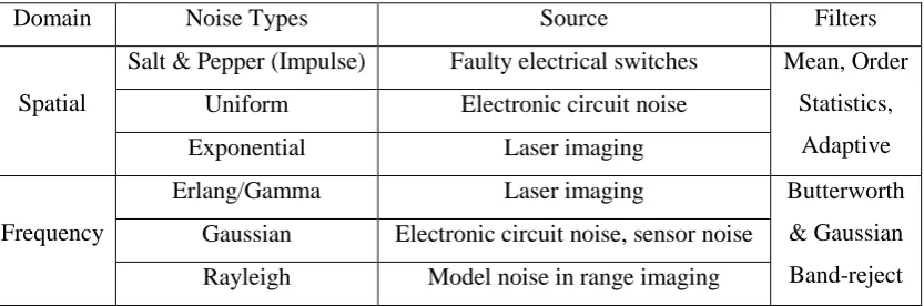
[image:24.595.113.530.429.567.2]For systemic noise, there are six known noise models, namely salt & pepper (impulse noise), Uniform, Exponential, Erlang, Gaussian and Rayleigh. Half of the mentioned noise has the characters of spatial noise, while the other three are periodic noise (Gonzalez & Woods, 2002). Table 2.1 is a summary of noise models, sources of those noise and the existing filters that can be used to filter them.
Table 2.1: Noises and their filters (Gonzalez & Woods, 2002)
Domain Noise Types Source Filters
Spatial
Salt & Pepper (Impulse) Faulty electrical switches Mean, Order
Statistics,
Adaptive Uniform Electronic circuit noise
Exponential Laser imaging
Frequency
Erlang/Gamma Laser imaging Butterworth
& Gaussian
Band-reject Gaussian Electronic circuit noise, sensor noise
Rayleigh Model noise in range imaging
Impulse noise is found in situations where faulty switching takes place during imaging; Exponential and Gamma densities mostly produce in laser medical imaging; Gaussian noise arises due to poor illumination or sudden high temperature; Rayleigh noise is useful for classification of noise phenomena in range imaging and finally, uniform noise density can be caused by electronic circuits. However, it is the least descriptive noise of practical situations (Gonzalez & Woods, 2002).
noise. Hence, image processing researchers combine and modify the existing filters to accommodate different noise types (Giannakeas and Fotiadis, 2009). Table 2.2 presents the existing noise filters for spatial and frequency domain. Spatial domain filters are used to remove random noise while frequency domain filters are useful to remove periodic noise.
Table 2.2: Spatial and frequency domain noise filter (Gonzalez & Woods, 2002)
Noise Filter Domain Filter Name Description
Spatial Arithmetic Mean Filter
Calculate average of pixels
Simple smoothing filter
Blurs image to remove noise
Order Statistics Filter
Based on ranking order of pixel
values
Useful filters include Median
Filter and Min & Max Filter
Adaptive Filter
Handles dense impulse noise
Smoothes non-impulse noise
Preserves details
Frequency
Butterworth Band-reject Filter Also known as band-pass filter
Allows a specified band of
frequencies pass through the
filter, discard the rest
Combination of low-pass and
high-pass filter Gaussian Band-reject Filter
Common noise that affects microarray images is impulse, Gaussian and periodic (frequency) noise. The filters that researchers use for those noise elimination are arithmetic mean (median filter) and two frequency domain filter; Fourier Transform filter and band-rejection filter (Gonzalez & Woods, 2002). These
2.4.1 Impulse Noise Removal using Median Filter
For impulse noise or salt and pepper noise, each pixel in an image has the probability
of fifty percent being contaminated either by white dot (salt) or black/dark dot (pepper). However, in some applications, noisy pixels are not simply black or white, which complicates impulse noise removal. The method for removing impulse noise is by using median filter. This filter simply rearranges all pixel values in ascending number (from 0 to 255), limited on the set area of pixel around the noise. From the arrangements of number, a median value is simply chosen to replace the noise value. The noise location can be detected in two ways physically, namely by detecting the black and white dots, or detection using pixel value, where noise pixels usually have sudden change of values either too high (255) or too low (0) while normal pixels values should have slight value difference to its adjacent pixel values.
The advantages of median filter are their abilities to effectively suppress the noise because median is the intermediate value that can tackle black (minimum value) and white (maximum value) dots. However, the disadvantages of the filter are that it affects clean pixels and causes noticeable edge blurring of original image (Gonzalez & Woods, 2002). Furthermore, Arias-Castro and Donoho (2009) claimed that generally, the Median-filtering theorem is false except cases where noise level per pixel is insignificant.
2.4.2 Additive White Gaussian Noise Removal
deionise Gaussian noise, which are the 2 dimensional convolution filters and the discrete Fourier transform filter.
The Fourier transform filter is invented by Tukey and Cooley in 1965 which is based on the basic idea of divide and conquer (Gonzalez & Woods, 2002). Fourier series is any function that periodically repeats itself, can be expressed as the sum of sines and/or cosines of different frequencies, where each component is multiplied by a different coefficient. Meanwhile for Fourier transform, functions are not periodic and can be expressed as the integral of sines and/or cosines multiplied by a
weighting function. Two dimensional Fourier transform is used because the first dimension is by transforming horizontally (row) and the second dimension is vertically (column). The two basics of Fourier transform are low-pass filter and high-pass filter and the effect of each filter is that low-high-pass filter produces brighter range of images as compared to high-pass filter. Depending on the original image used, commonly high-pass filter has higher contrast between the objects against the background, hence high-pass filter can be used and hybridised with different algorithms to enhance images. Meanwhile low-pass filters are commonly used for smoothing images with choices of several standard forms such as ideal low-pass filter, Butterworth low-pass filter and Gaussian low-pass filter. The filters work by cutting off all high frequency components of the Fourier transform that are at a distance larger than a specified value.
The advantages of this noise removal is that it yields real value output image and also do a fast transform, hence it is usually used for image compression. The disadvantages of Fourier transform are that it has bad convergence property and without time information, even when the domain used for the transform is frequency (Gonzalez & Woods, 2002). In 2010, Adamczak et al. claimed that the Fourier Transform Filter is very useful for analysing and denoising periodic signals. However, when additional ‘scratch’ and disturbances are introduced into the signals,
the signals become unstable and Fourier Transform must rely on other filter to
2.4.3 Periodic Noise Removal using Band-rejection Filter
The last filter to be discussed is the periodic noise remover that is obviously going to combat with periodic noise. It is the noise which shows in a specific manner of frequency. Commonly, the filters used are band-rejection and Notch filters. These filters work with noise from electrical or electromechanical interference that occur during image acquisition. The advantages are, periodic noise is spatially independent and can easily be observed in frequency domain (because it is periodic). The idea behind the periodic noise filter is simply suppressing noise component in the frequency domain.
The developed filters prove that noise reduction is an essential process even
there is endless possibilities of what filter combination can be used to remove noise. Abundant of image denoising techniques have been suggested by researchers.
However, there are inadequate suggestions and research on microarray image denoising. Researches for microarrays have only focused mainly on finding accurate spot gridding and segmentation (Gonzalez & Woods, 2002; White et al., 2005; Deepa & Thomas, 2009). Unlike other researchers, Manjunath (2014) referred his denoising stage as restoration stage because in his work, instead of just removing noise generally, he identifies the noise and its characteristics first before removing them. In doing this way, he ‘reverses’ the noise effect which later ensures that the essential information is preserved.
2.4.4 Previous Works in Microarray Denoising
Here gives brief overview of some methods that are developed successfully for microarray image denoising. Manjunath (2014) proposed novel techniques for image pre-processing / restoration. He developed a restoration system model which firstly takes the noisy image as input, and next he estimated the type of noise
Zacharia and Maroulis(2011) have proposed a noise resistant approach which works well even under the adverse conditions, when there is an appearance of various spot shapes, (volcano shaped and doughnut shaped spots). When the intensities of the spots are diverse, such as low intensity spots (not clearly visible) and spots are saturated, the approach discussed is robust in extracting the foreground signal. The approach is also fully automated and does not need any human intervention to find the contour of microarray spots. It has been tested on synthetic spots and real spots which are aided with fuzzy logic to handle the uncertainties caused by the noise. The
results prove that the method is efficient against other traditional segmentation methods that rely on two-dimensional segmentation.
Meher et al. (2011) developed two novel pre-processing techniques, namely optimized spatial resolution and spatial domain filtering. Spatial filtering is used for denoising of microarray image while spatial resolution optimization is used to enhance the image for accurate quantification of the spots. In order to improve the quantification results, an integrated spatial domain filtering (SDF) and optimized spatial resolution (OSR) have been used. For OSR, the density of pixels over the image is used. The greater spatial resolution, the more pixels are used to display the image. It is found that pixel intensities of the microarray appear in a particular order in alternate rows. Next for SDF, the method works by moving a rectangular mask of the order m by n over the given microarray image. The mask is called filter. A linear filter can be implemented by multiplying all the elements in the mask by corresponding elements in the area spanned by filter mask adding together of all these products. From the findings, the method is proven simple and speed up real-time processing. Additionally, the integrated OSR-SDF shows much higher spot intensity as compared to the single approach of OSR.
Meher et al. also proves that images can be pre-processed spatially using
the signal or the histogram of the image, instead of directly applying filters onto the image itself. Meanwhile, Manjunath implants the idea of recognising type of noise
pre-processing step of microarray image analysis. Therefore, techniques which depends exclusively on the image characteristics, is proposed in this research work.
2.5 Microarray Spot Gridding
Spot gridding algorithms are divided into three classes, according to the degree of human intervention in the process and they are manual gridding, semi-automatic gridding and automatic gridding.
Manual gridding was the first method used in early days of microarray technology. It is time-consuming and tiring as it can takes up to days, which can lead to human errors. According to Draghici (2003), manual spot finding is essentially relying on computer aid because it is not able to detect the spots by itself. Computers merely provide tools to allow users to detect the signals of the image. This was the first method used in microarray technology, which is very time consuming and requires intensive labour to detect thousands of spots. Users also have to manually adjust the circles over the spots until a considerable level of accuracy is accepted. This method is recognised as the poorest method due to human errors, irregular array spacing and large variation of spot sizes.
The second method is semi-automatic gridding, which typically uses algorithms to adjust spot location automatically after human guidance. Usually a user is required to click the topmost and leftmost spot which is the approximation location of the grid. The algorithm later produces an outline of the estimated the spots and later, human intervention involves to correct any inaccurate outlines. User interface tools are usually provided by software to assist him/her to manually adjust
the grids if the algorithm fails to do so. This method is better in time saving as compared to manual gridding and is not too tedious as the user only needs to do only
minor adjustment to spot location, if required (Draghici, 2003).
which is red, green and yellow. Usually, researcher modifies the technique and algorithm so they can work well with sampled data they already have. The parameters related to addressing include margin between grids, margin between spots, individual coordinate of spots and the rotation of the microarray. Rotation is considered to be important because slight miss registration of rotation may cause entire spot wrongly addressed and the subsequent steps would be prone to errors (Meher et al., 2011). The process of finding grids of spots rely on margins, but this parameter is usually negatively affected by noise, and thus a sequence of detailed
gridding framework requires both pre-processing and grid processing.
2.5.1 Previous Works in Microarray Spot Gridding
Manjunath (2014) proposed three methods for microarray gridding stage. Based on his proposed system flow, the input image is raw and expected to be misaligned (skewed) and affected by noise. Next, the image undergoes skew detection and correction. The first method proposed is Spatial Topology Method which literally means spatial is something related to space, and topology is the study of geometrical properties and spatial relations; specifically central to mathematical area (Manjunath, 2014).
He defined spatial topology that is actually the pixel values of the connected component; utilising properties of the coloured spot (foreground) gives positive numbered value while its dark background are valued zero. The differences are calculated for each connected component, where if there is an abrupt or sudden change of value, shows that it is the end of previous row of spots and beginning of the next row of spots. The gridlines are generated from the average values between spots which indicate the middle location that separates between spots. The methods proposed resulted to have execution time proportional to the number of spots and the noise level, meaning that the methods consume more processing time for noisy images. The noisier the image gets, the slower the processing time is.
modification of pixel intensity profile (also known as image signal). The work also consists of refinement procedures to enhance OMTG to detect spots despite the noise. However, among the successful spot gridded, there are several issues that OMTG is unable to conquer, which is OMTG’s weakness against spilled dyes which were found by biologist during microarray creation experiment (refer to Figure 2.2).
Figure 2.2: OMTG failure to detect region of some spots (Rueda & Rezaian, 2011)
The previous works have presented the usefulness of image signal as a precise spot location detector. This is possible if the threshold contrast between spots, noise and background is distinguishable. Hence, the spot gridding stage of microarray analysis is still relying on a successful denoising stage, so that a successful isolated ‘spot’ is not actually a noise. The stubborn noise that cannot simply be removed and reversed using common noise filters includes experimental noise that occurs during biological procedures. Besides that, the class of human intervention in gridding is also questionable: ‘Is fully automatic gridding really useful and saves time?’
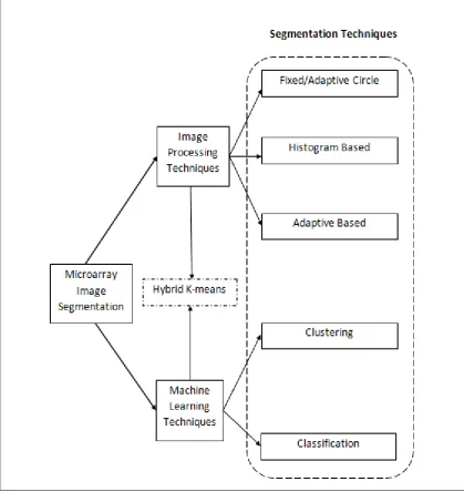
2.6 Microarray Spot Segmentation
After microarray locations are gridded, the spots will be segmented. The summary of microarray image segmentation methods by Giannakeas and Fotiadis, (2009) where it is classified into three segmentations, namely fixed/adaptive circle segmentation, histogram based segmentation and adaptive shape segmentation (refer to Figure 2.3). Under these three methods of segmentations, there are many existing software/algorithms by other researchers such as Scanalyse and Genepix (under Affymetrix Company). The software is under fixed/adaptive circle segmentation, while QuantArray and Mann-Whitney Test are under histogram based segmentation. Finally, seed-region growing and watershed transform are under adaptive shape segmentation. Meanwhile for segmentation using machine learning techniques are Fuzzy C-Means, Expectation Maximisation and Bayes Classifier (Giannakeas & Fotiadis, 2009). Overview of each of the segmentations methods; fixed/adaptive circle segmentation, histogram based segmentation and adaptive shape segmentation
are discussed as follows.
Eisen and Brown (1999) have claimed that Fixed Circle algorithm is one of
Ruusuvuori & Yli-Harja, 2006). Fixed Circle segmentation algorithm is implemented in several microarray software such as Magic Tool (Heyer & Akin, 2005), and Scan Alyze (Eisen & Brown, 1999).
Histogram/Intensity based image segmentation (HBS) can be obtained through four methods which are Histogram based method (Thresholding), Edge-based method, Region-Edge-based method and Model-Edge-based method (Kumar et al., 2009). The main idea of thresholding is to classify pixels into its group with respect to certain similarity, such as the intensity level of pixels. Threshold technique evaluates
each pixel producing black and white images where the group of pixels of interest are indicated with white. Meanwhile, the remaining pixels are indicated by black and become the background (Kaur & Singh, 2011). HBS Thresholding can be divided into Global Thresholding (GT) and Local Thresholding. Thresholding pixel of an image can be based on several features like the histogram, mean, standard deviation or gradient. When only one threshold is selected for the whole image, it is a ‘global’
thresholding. Meanwhile if thresholding only rely on say local average gray value, then it is a ‘local’ thresholding. If a local thresholding is selected independently for each group of pixels, it is called as ‘adaptive’ technique.
Figure 2.3: Microarray spot segmentation methods (Giannakeas & Fotiadis, 2009)
2.7 Existing Microarray Architecture Analysis
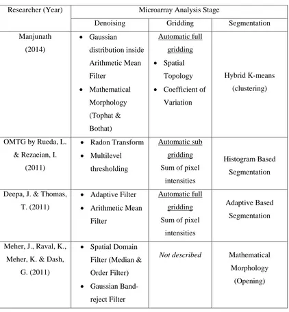
Several techniques for microarray analysis used by image processing researchers were classified into three stages, namely the pre-processing (for noise removal), gridding (for locating individual spot) and segmentation (to extract the spot). All these researches are summarised as shown in Table 2.3.
onto pixel projection to locate spots. Researchers who also used pixel intensity projection to locate spot location were Nagesh et al. (2010), Siswantoro (2010) and Deepa & Thomas (2009). All of them used pixel projection but applied different techniques to extract or manipulate the projection. However, Meher et al. (2011) used pixel projection in pre-processing stage and its technique is named as Optimized Spatial Resolution. Besides that, Chen et al. (2006) used Kernel Density Estimation to manipulate pixel projection and they applied it for segmentation stage instead of gridding stage.
Table 2.3: Summary review of existing microarray analysis architecture
Researcher (Year) Microarray Analysis Stage
Denoising Gridding Segmentation
Manjunath (2014) Gaussian distribution inside Arithmetic Mean Filter Mathematical Morphology (Tophat & Bothat) Automatic full gridding Spatial Topology
Coefficient of
Variation
Hybrid K-means
(clustering)
OMTG by Rueda, L.
& Rezaeian, I.
(2011)
Radon Transform
Multilevel
thresholding
Automatic sub
gridding
Sum of pixel
intensities
Histogram Based
Segmentation
Deepa, J. & Thomas,
T. (2011)
Adaptive Filter
Arithmetic Mean
Filter
Automatic full
gridding
Sum of pixel
intensities
Adaptive Based
Segmentation
Meher, J., Raval, K.,
Meher, K. & Dash,
G. (2011)
Spatial Domain
Filter (Median &
Order Filter)
Gaussian
Band-reject Filter
Not described Mathematical
Morphology
Table 2.3: Summary review of existing microarray analysis architecture (continued)
Researcher (Year) Microarray Analysis Stage
Denoising Gridding Segmentation
Nagesh, S., Varma,
S. & Govardhan, A.
(2010) Adaptive Filter (Weiner Filter) Automatic sub gridding Mean Intensity Profile Mathematical Morphology
Adaptive Based
Segmentation
(Watershed &
Iterative
Watershed)
Siswantoro, J.
(2010) Not conducted
Automatic full
gridding
Pixel Profile
Not conducted
Kakumani, A.,
Mendhuwar, A. &
Kakumani, R. (2010)
Independent
Component Analysis
Filter (smoothing)
for Gaussian noise
Not conducted Not conducted
Ni, S., Wang, P.,
Paun, M., Dai, W. &
Paun, A. (2009)
Not conducted Not conducted
Adaptive Based
Segmentation
Deepa, J. & Thomas,
T. (2009)
Adaptive &
Arithmetic Mean Filter Mathematical Morphology (Opening) Automatic sub gridding Pixel Intensity Profile Not conducted ARMADA by Chatziioannou, A.,
Moulos, P. &
Kolisis, F.
(2009)
Background
correction
Spot quality
filtering Normalisation Semi-automatic full gridding Trust Factor Calculation Not conducted
be used for all stages of microarray analysis, from pre-processing to segmentation. Besides that, Nagesh et al. (2010) and Deepa & Thomas (2009) applied mathematical morphology exclusively for pre-processing stage which both researchers have proved that morphological operation is reliable to be used either in single or combined forms. Several other techniques that can be used for pre-processing include gradient based method (Kakumani et al., 2010) and histogram based method (Deepa & Thomas, 2011). An architecture developed by a team of biologists named Automated Robust MicroArray Data Analysis (ARMADA)
consists of pre-processing, gridding, data extraction and clustering tools.
In Table 2.3, the trend shown by computer researchers includes applying mathematical morphology and pixel intensity profiles into stages of microarray analysis. This allows potential of techniques to have flexibility of modification, where some researchers applied it on image, while some applied it on the signal of the image. It is flexible to apply into any stages of microarray analysis and finally gets good reliability, where researchers have done ongoing researches on these techniques for years.
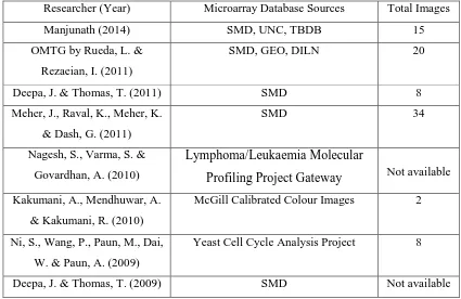
Architectures mentioned in the same table tested the architecture’s compatibilities in several microarray databases, because different databases feature different characteristics of microarray. Different manufacturers and biologists submitted different sizes of microarrays (row and column number), colour types and experimental background. The lists of microarray database sources used by other researchers are listed as in Table 2.4. Most databases are available online, such as Stanford Microarray Database (SMD), University of North Carolina (UNC), Gene Expression Omnibus (GEO), Tuberculosis Database (TBDB), Lymphoma/Leukaemia Molecular Profiling Project Gateway, McGill Calibrated Colour Images and Yeast Cell Cycle Analysis Project. Dilution experiment
microarrays (DILN) can be requested from Ramdas et al. (2001).
Apart from the applications and techniques developed by computer
a user has in his/her working station. Meanwhile, AMIA is a toolbox that must be used with MATLAB and facilitates people without programming skills.
Table 2.4: Microarray database used by other architectures
Researcher (Year) Microarray Database Sources Total Images
Manjunath (2014) SMD, UNC, TBDB 15
OMTG by Rueda, L. &
Rezaeian, I. (2011)
SMD, GEO, DILN 20
Deepa, J. & Thomas, T. (2011) SMD 8
Meher, J., Raval, K., Meher, K.
& Dash, G. (2011)
SMD 34
Nagesh, S., Varma, S. &
Govardhan, A. (2010)
Lymphoma/Leukaemia Molecular
Profiling Project Gateway Not available Kakumani, A., Mendhuwar, A.
& Kakumani, R. (2010)
McGill Calibrated Colour Images 2
Ni, S., Wang, P., Paun, M., Dai,
W. & Paun, A. (2009)
Yeast Cell Cycle Analysis Project 8
Deepa, J. & Thomas, T. (2009) SMD Not available
ARMADA and AMIA differ slightly from the previous mentioned
REFERENCES
Adamczak, R., Litvak, A., Pajor, A., & Tomczak-Jaegermann, N. (2010).Quantitative Estimates of the Convergence of the Empirical Covariance Matrix in Log-Concave Ensembles. Journal of the American Mathematical Society, 23(2), 535-561.
Angulo, J. (2008). Polar Modelling and Segmentation of Genomic Microarray Spots using Mathematical Morphology. Image Analysis and Stereology, 27 (2), 107-124.
Arias-Castro, E., & Donoho, D. L. (2009). Does Median Filtering Truly Preserve Edges Better Than Linear Filtering? The Annals of Statistics, 1172-1206.
Athanasiadis, E., Cavouras, D., Spyridonos, P., Glotsos, D., Kalatzis, I., & Nikoforidis, G. (2007). Segmentation Of Microarray Images Using Gradient Vector Flow Active Contours Boosted By Gaussian Mixture Models. Second International Conference on Experiments/Process/System Modeling/Simulation/Optimization
(2nd IC-EpsMsO), July 4th--7th, Athens, Greece.
Bajcsy, P. (2004). Gridline: Automatic Grid Alignment DNA Microarray Scans. Image
Processing, IEEE Transactions on, 13 (1), 15-25.
Bariamis, D., Maroulis, D., & Iakovidis, D. K. (2010). Unsupervised SVM-based Gridding for DNA Microarray Images. Computerized Medical Imaging and
Graphics, 34 (6), 418-425.
Blekas, K., Galatsanos, N. P., Likas, A., & Lagaris, I. E. (2005). Mixture Model Analysis of DNA Microarray Images. Medical Imaging, IEEE Transactions on , 24 (7), 901-909.
Brandle, N. B., & Lapp, H. (2003). Robust DNA Microarray Image Analysis. Machine
Vision and Application, 15, pp. 11-28.
Canny, J. (1986). A computational approach to edge detection. Pattern Analysis and
Machine Intelligence, IEEE Transactions on, (6), 679-698.
Chen, W. B., & Liu, W. L. (2006). An Automated Gridding and Segmentation Method for cDNA Microarray Image Analysis. Computer-Based Medical Systems,
2006. CBMS 2006. 19th IEEE International Symposium on, (pp. 893-898).
Compumine. (2012). Evaluating a Classification Model - Precision and Recall tell me? Tech. rep., Old Diminion University.
Cooley, J. W., & Tukey, J. W. (1965). An Algorithm for the Machine Calculation of complex Fourier series. Mathematics of computation, 19(90), 297-301.
Deepa, J., & Thomas, T. (2009). Automatic Gridding of cDNA Microarray Images using Optimum Subimage. International Journal of Recent Trends in
Engineering, (pp. 37-40).
Deepa, J., & Thomas, T. (2011). A Robust Method for Extracting Features from Noisy Microarray Images. International Journal of Research and Reviews in
Computer Science.
Dozmorov, I., & Lefkovis, I. (2009). Internal Standard-based Analysis of Microarray Data. Part 1: Analysis of Differential Gene Expressions. Nucleic Acids
Research, 37, pp. 3578-3579.
Draghici, S. (2003). Data Analysis Tools for DNA Microarrays. Florida: Chapman & Hall.
Edgar, R. D., & Lash, A. E. (2002). Gene Expression Omibus: NCBI Gene Expression and Hybridization Array Data Repository. Nucleic Acids Research, 30, pp. 207-210.
Efford, N. (2000). Digital Image Processing: A Practical Introduction using Java (with
CD-ROM). Addison-Wesley Longman Publishing Co., Inc.
Eisen, M. B., & Brown, P. O. (1999). DNA arrays for analysis of gene expression. Methods in Enzymology, 179-204.
Fisher, R. P., & Wolfart, E. (2003). Erosion and Dilation. Hypermedia Image
Processing Reference .
Fraser, K. W. (2007). Noise Filtering and Microarray Image Reconstruction via Chained Fouriers. Advances in Intelligent Data Analysis VII (pp. 308-319). Springer Berlin Heidelberg.
Giannakeas, N., & Fotiadis, D. I. (2009). An Automated Method for Gridding and Clustering-based Segmentation of cDNA Microarray Images. Computerized
Medical Imaging and Graphics, 33 (1), 40-49.
Gonzales, R., & Woods, R. (2002). Digital Image Processing Second Edition. Digital
Hang, X., & Wu, F. X. (2009). Sparse representation for classification of tumors using gene expression data. BioMed Research International, 2009.
Heyer, L. J., & Akin, B. (2005). MAGIC Tool: Integrated Microarray Data Analysis.
Bioinformatics, 21 (9), 2114-2115.
Hirata, R.,Barrera, J., Hashimoto, R. and Dantas, D.. (2001). Microarray gridding by mathematical morphology. Brazilian Symposium on Computer Graphics and Image Processing. 14 (1), p1-8.
Kakumani, A., Mendhurwar, K. A., & Kakumani, R. (2010). Microarray Image Denoising using Independent Component Analysis. International Journal of
Computer Applications.
Karimi, N. S., & Behnamfar, P. (2010). Segmentation of DNA Microarray Images using An Adaptive Graph-based Method. IET image processing, 4 (1), 19-27.
Kaur, G., & Singh, B. (2011). Intensity Based Image Segmentation using Wavelet Analysis and Clustering Techniques. Published in IJCSE, Indian Journal of
Computer Science and Engineering, 2 (3).
Kumar, H. C., Raja, K. B., Venugopal K. R. and Patnaik, L. M. (2009) Automatic Image Segmentation using Wavelets. IJCSNS International Journal of
Computer Science and Network Security, 9(2).
Labib, E., Fouad, I., Mabrouk, M., & Sharawy, A. (2012). An Efficient Fully Automated Method for Gridding Microarray Images. American Journal of
Biomedical Engineering, 2 (3), 115-119.
Lapedes, D. N. (1978). McGraw-Hill Dictionary of Scientific and Technical Terms. (D. N. Lapedes, Ed.) McGraw-Hill New York.
Larese, M. G., & Juan, C. (2009). Quantitative Improvements in cDNA Microarray Spot Segmentation. In Advances in Bioinformatics and Computational Biology (pp. 60-72). Springer.
Lehmussola, A., Ruusuvuori, P., & Yli-Harja, O. (2006). Evaluating the performance of microarray segmentation algorithms. Bioinformatics, 22(23), 2910-2917.
Lipori, G. (2005). Efficient gridding of real microarray images. In Proceedings of the Workshop on Biosignal Processing and Classification of the International Conference on Informatics in Control, Automation and Robotics.
Mathworks Product Documentation. (2009). Morphology fundamentals: dilation and erosion. Retrieved from http://www.mathworks.com/help/toolbox/images/f18-12508.html.
Meher, J. R., & Dash, G. (2011). The Role of Combined OSR and SDF Method for Pre-Processing of Microarray Data That Accounts for Effective Denoising and Quantification. Journal of Signal and Information Processing, 2 (03), 190.
Nagesh, A. S., Varma, D. G., & Govardhan, D. A. (2010). An improved iterative watershed and morphological transformation techniques for segmentation of microarray images. IJCA Special Issue on “Computer Aided Soft Computing Techniques for Imaging and Biomedical Applications” CASCT, 2, 77-87.
Namee, B. M. (2007). Image Restoration: Noise Removal. Image Restoration: Noise
Removal .
National Instruments (2013). Peak Signal-to-Noise Ratio as an Image Quality Metric.
Ni, S. H., Wang, P., Paun, M., Dai, W., & Paun, A. (2009). Spotted cDNA microarray image segmentation using ACWE. Romanian Journal of Information Science and Technology, 12(2), 249.
Ortiz, F., Torres, F., De Juan, E., & Cuenca, N. (2002). Colour mathematical morphology for neural image analysis. Real-Time Imaging, 8(6), 455-465.
Pollack, J. R. (2007). A perspective on DNA microarrays in pathology research and practice. The American journal of pathology, 171(2), 375-385.
Ramdas, L., Coombes, K. R., Baggerly, K., Abruzzo, L., Highsmith, W. E., & Krogmann, T. Z. (2001). Sources of Nonlinearity in cDNA Microarray Expression Measurements. Genome Biology 2, (pp. 1-7).
Rochester Medical Center (2012). DNA Microarrays (Gene Chips) and Cancer. DNA Microarrays (Gene Chips) and Cancer , Life Sciences Learning Center.
Rueda, L. (2008). An Efficient Algorithm for Optimal Multilevel Thresholding of Irregularly Sampled Histograms. In Structural, Syntactic, and Statistical Pattern Recognition (pp. 602-611). Springer Berlin Heidelberg.
Rueda, L., & Rezaeian, I. (2011). A Fully Automatic Gridding Method for cDNA Microarray Images. BMC Bioinformatics, 12, p. 113.
Sánchez, A., and Villa, M. C. R.(2008) A Tutorial Review of Microarray Data Analysis.
Bioinformatics Tutorial. Universitat de Barcelona.
Scherer, A. D., & Meng, F. (2013). Impact of Experimental Noise and Annotation Imprecision on Data Quality in Microarray Experiments. Statistical Methods
Scientific Volume Imaging. (2014). Image Histogram. Image Histogram . Netherlands.
Sherlock, G., Hernandez-Boussard, T., Kasarskis, A., Binkley, G., Matese, J. C., Dwight, S. S., et al. (2001). The Stanford Microarray Database. Nucleic Acids Research, 28.
Siegrist, K. (1997). The Rayleigh Distribution. Tech. rep., University of Alabama.
Siswantoro, J. (2010). Automatic Gridding for DNA Microarray Image Using Image Projection Profile. Proceedings of the 6th Conference on Mathematics,
Statistics and its Applications.
Smith, S. W. (2011).Chapter 25: Special Imaging Techniques / Signal-to-Noise Ratio’. The Scientist and Engineer’s Guide to Digital Signal Processing. California
Technical Publishing.
Solomon, C., & Breckon, T. (2011). Fundamentals of Digital Image Processing : A
Practical Approach with Examples in MATLAB. West Sussex:
Wiley-Blackwell.
Thompson, C. M. & Shure, L. (1995). Image Processing Toolbox: For MATLAB.Mathworks Documentation.
Valarmathi, S. S., & Balasubramaniam, S. (2012). Noise Reduction from the Microarray Images to Identify the Intensity of the Expression. Proceedings of the Second International Conference on Soft Computing for Problem Solving (pp. 1451-1465). Springer India.
Vergara, J. P., & Watson, L. T. (2008). GridWeaver: A Fully-Automatic System for Microarray Image Analysis using Fast Fourier Transforms.
Wang, Y., Shih, F., & Ma, M. (2005). Precise gridding of microarray images by detecting and correcting rotations in subarrays. In Proceedings of the 8th Joint Conference on Information Sciences (pp. 1195-1198).
White, A. M., Daly, D. S., Wilse, A. R., Protic, M., & Chandler, D. P. (2005). Automated Microarray Image Analysis Toolbox for MATLAB.
Bioinformatics, (pp. 3578-3579).
Yang, Y. H., Buckley, M. J. & Speed, T. P. (2001). Analysis od cDNA Microarray Images. Briefings in Bioinformatics, (pp. 341-349).
Zacharia, E., & Maroulis, D. (2011). A Spot Modelling Evolutionary Algorithm for Segmenting Microarray Images. Evolutionary Algorithms, (pp. 480-495).