© 2017, IRJET | Impact Factor value: 5.181 | ISO 9001:2008 Certified Journal | Page 494
Jaya with Experienced Learning
Prasenjit Baruah
1UG-Student,Dept.of
Production Engineering,N.I.T Tiruchirapalli,Tiruchirapalli,India
---***---Abstract -
Jaya Algorithm has emerged as a simple but themost effective approach in the field of engineering optimization and beyond. Unlike the conventional heuristic algorithms like PSO, GA, etc, it doesn't require any algorithm specific parameters. A modified version of the Jaya Algorithm has been proposed in this paper that can be used for solving constrained and unconstrained problems. Jaya tried to learn only from the 'best and the 'worst' of the candidate solutions. Such combination is expected to have biasness and may result local optimal. In order to avoid this, it is proposed in the modified Jaya to seek additional guidance from one each from the top and the bottom most 10% candidate solutions when endeavoring to look for improvement in subsequent iterations. The performance of the proposed algorithm is observed by implementing it on 5 test functions having different characteristics and the results obtained show much better results as compared to that from existing Jaya Algorithm.
Key Words: Optimisation, Jaya, Evolutionary Approaches, Endeavouring, Iterations.
1. INTRODUCTION
Optimization is basically seeking for the best or most effective use of a resource. In the field of Engineering, various optimization techniques have been employed to solve real life problems like cost reduction, scheduling, etc. The population based heuristic algorithms have two approaches: Evolutionary and Swarm Intelligence. As this paper deals with the modification of recently evolved random search algorithm 'Jaya', the concepts involved in the predecessors like TLBO, PSO, GA, etc have contributed greatly to understand the origin of the same.
PSO:- This Algorithm is based on the behavior of a flock of birds searching for food in a particular search space. These particles(i.e. candidates solutions) are moved around in the search space as per some formula. They are guided by their respective best solution in the search space(i.e. pbest)
as well as the entire swarm's best known position(i.e. gbest). Thus it takes both its own solution and the leader's
solution(i.e. most experienced) into account while searching for the optimal solution.
TLBO:- With the advent of TLBO, a parameter less optimization approach which gained great acceptance among the researchers, people started analyzing natural phenomenon to improve the random search and optimization techniques. TLBO replicates the events taking place inside a classroom. It consists of 2 phases -The Teacher Phase and -The Learner's Phase. What happens in a classroom is the students(i.e. learners) gain knowledge in two ways! Either from what he has been taught by the teacher or by the mutual interaction with his fellow mates. Now the Teacher, being the most learned is considered as the 'best' solution. However, the learning capacity of every individual may be different. After gaining knowledge from the 'best', the students get themselves involve in group discussions where they interact with others and try to improve their knowledge.
JAYA:- It is a new random search optimization algorithm which is similar to TLBO in terms of consideration of parameters. But unlike TLBO, it has only one phase in which the solutions are moved towards the best by avoiding the worst. The success of this algorithm is due to the fact that it takes the worst solution into account while trying to improve each solution. Owning to its victorious nature, it has been named 'Jaya' which is a Sanskrit word meaning victory.
© 2017, IRJET | Impact Factor value: 5.181 | ISO 9001:2008 Certified Journal | Page 495
1.1 Model
Let's take the situation of occurrence of a natural calamity like Earthquake. The population near the epicenter would be the worst affected whereas the population far away from it would be safe and least affected(i.e. Best). However, the population in between these extremities will try to rush to an immediate safer place in reaction to the trembling .So, the concept of information flow must be continuous and versatile. It is beneficial to take guidance from both the individuals which are close to the Best and the Worst in addition to the two(i.e. Best & Worst).
Blue Dots--No. of Candidates(say 20).
The encircled region shown in figure corresponds to Top 10% near Best and Bottom 10% near Worst.10% of 20 is 2,there are 2 candidates each in addition to the Best and the Worst.
Now the remaining candidates between the two extremities will try to rush out to an immediate better place by taking guidance from anyone who are in the encircled region following the equations-
(#)x' = x + rand(xtop - |x|) - rand(xbottom -
|x|)...towards top 10% and away from the bottom 10%
After taking guidance from the candidates within the marked regions , we seek guidance from the Best and the Worst as these are regarded as the most experienced to get finer results.
2. PROPOSED ALGORITHM
Let f(x) is the objective function to be minimized(or maximized). At any iteration i, assume that there are n number of candidates (population size, i.e. (i.e. k=1,2,3,...,n) ) and m number of design variables (i.e. j=1,2,3,...,m). Let the best candidate obtains the best value of objective function(f(x)best) and the worst candidate obtains the worst value of objective function(f(x)worst) in the entire candidate solution. Rank each candidate according to the objective function value. Obtain 10% of the population size and extract the values near the Best and the Worst solutions respectively. Select two random solutions each among the Top 10% and the Bottom 10% and modify each solution as per the following the equation:
x' = x + rand(xtop - |x|) - rand(xbottom - |x|)...towards top
10% and away from the bottom 10%.
where, xtop = randomly chosen number from top 10%,
xbottom = randomly chosen number from bottom 10%. x' is
the new value of x and rand is a random number in the range[0 1]. The term "rand(xtop - |x|)" sets the direction of the candidates' solutions towards the neighborhood of the Best. Whereas the term "- rand(xbottom- |x|)" sets the
direction of the candidates' solutions away from the neighborhood of the Worst.
Ultimately, the candidates would seek guidance from the most experienced candidates that are the Best and the Worst. Therefore, the candidate solutions in the previous step are modified according to the Jaya equation which allows already oriented solutions to refine and gain the desired the result. The Jaya equation goes as follows :
x' = x + rand(xbest - |x|) - rand(xworst - |x|)
Fig.1 shows the flowchart of the proposed algorithm. The algorithm always tries to get closer to success (i.e. reaching the best solution) and tries to avoid failure (i.e. moving away from the worst solution) gaining knowledge from the neighborhood. The algorithm strives to become successful by reaching the best solution in less number of iterations as compared to its parent algorithm(i.e. Jaya Algorithm) and hence it is modified. The proposed method is illustrated by means of an unconstrained benchmark function known as Sphere function in the next section.
© 2017, IRJET | Impact Factor value: 5.181 | ISO 9001:2008 Certified Journal | Page 496
unconstrained benchmark function of Sphere isconsidered. The objective function is to find out the values of xi that minimize the value of the Sphere function. min f(x)=∑xi2
subject to: -100<xi<100
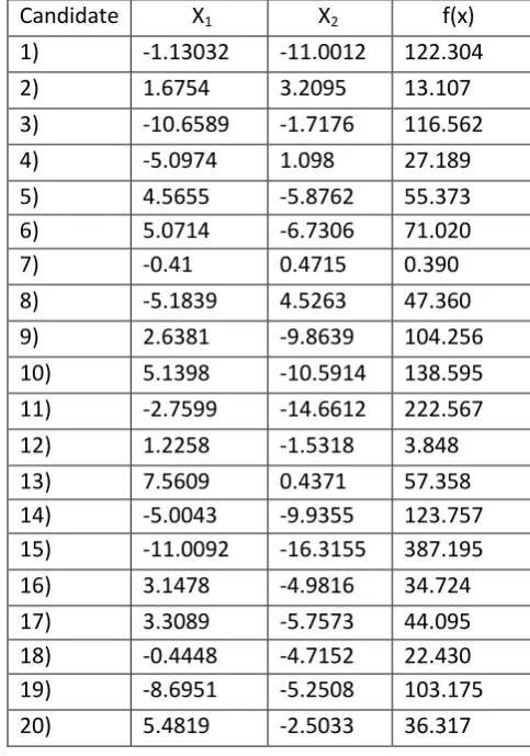
[image:3.595.322.564.321.666.2]Since the objective function is to be minimized, thus the minimum value of the given benchmark function is 0 for all xi values of 0.Now to demonstrate the modified Jaya algorithm, let us assume a population size of 20 (i.e. candidate solutions), two design variables x and y and two iterations as the termination criterion. The initial population is randomly generated within the ranges of the variables and the corresponding values of the objective function are shown in Table 1. As it is a minimization function, the lowest value of f(x) is considered as the best solution and the highest value of f(x) is considered as the worst solution.
Table -1: Initial Population
corresponding to Candidate 12 and the Worst solution is corresponding to Candidate 15. As we know 10% of 20 candidates in 2 thus we obtain two solutions each near the Best and near the Worst. Then we choose any random number from each two solutions to get rough direction. Rank 3- Candidate 16
Rank 18- Candidate 13
Now each value of x1 and x2 are modified so as to move towards the Top 10%(neighborhood of Best) and away from the Bottom 10%(neighborhood of Worst) according to the equation
[image:3.595.36.564.358.791.2]x' = x + rand*(x(top) - |x|) -rand*(x(bottom)-|x|)
Table 2:- Intermediate Values of x & y
Candidate X
1X
2f(x)
1)
-1.13032
-11.0012
122.304
2)
1.6754
3.2095
13.107
3)
-10.6589
-1.7176
116.562
4)
-5.0974
1.098
27.189
5)
4.5655
-5.8762
55.373
6)
5.0714
-6.7306
71.020
7)
-0.41
0.4715
0.390
8)
-5.1839
4.5263
47.360
9)
2.6381
-9.8639
104.256
10)
5.1398
-10.5914
138.595
11)
-2.7599
-14.6612
222.567
12)
1.2258
-1.5318
3.848
13)
7.5609
0.4371
57.358
14)
-5.0043
-9.9355
123.757
15)
-11.0092
-16.3155
387.195
16)
3.1478
-4.9816
34.724
17)
3.3089
-5.7573
44.095
18)
-0.4448
-4.7152
22.430
19)
-8.6951
-5.2508
103.175
20)
5.4819
-2.5033
36.317
Candidate X
1X
2f(x)
Rank
1)
-2
-8
68
13
2)
4
5
41
7
3)
-9
0
81
17
4)
-2
6
40
6
5)
8
-3
73
14
6)
6
-3
45
9
7)
0
7
49
11
8)
-4
5
41
7
9)
5
-7
74
15
10)
8
-6
100
19
11)
1
-8
65
12
12)
-1
-1
2
1
13)
8
5
89
18
14)
-4
-8
80
16
15)
-8
-9
145
20
16)
4
-1
17
3
17)
6
-3
45
9
18)
2
-1
5
2
19)
-6
0
36
4
20)
6
1
37
5
© 2017, IRJET | Impact Factor value: 5.181 | ISO 9001:2008 Certified Journal | Page 497
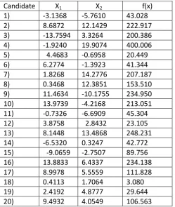
Table 3:- New values of the variables and the objectivefunction during first iteration by applying Jaya equation
Table 4:- Updated values of the variables and the objective function based on fitness comparison at the end of first iteration
Table 4 has been updated based on the fitness of the Objective function by comparing the values among Table 1,2 &3. Thus, the Updated table has values from all the 3 tables depending on the goal(i.e. minimization or maximization). It validates the fact that the candidates are acquiring information from the neighborhood of the Best and the worst too. In this way, it approaches the optimum result by executing the required number of iterations.
2.2Approach
The working of the proposed algorithm has been found out by comparing the results of the following four cases:
(1) Jaya Algorithm
(2) Jaya Algorithm + Top 10%(near the BestSol)
(3) Jaya Algorithm + Bottom 10%(near the WorstSol)
(4) Jaya Algorithm + Top 10% + Bottom 10%.
All the above mentioned algorithms have been coded in Matlab and the outcomes are compared on the basis of convergence rate and better results. For this purpose the objective function is taken as the Sphere function and the other parameters like range of design variables, max iterations, etc are kept constant.
No. of Candidates: 20
Design Variables: 2
Max Iterations: 100
Lower Bound: -100
Upper Bound: 100
It is observed that the results of the first two cases are almost similar(Fig(1) & Fig(2)). However, when a random candidate solution from the neighborhood of the Worst
is
Candidate X
1X
2f(x)
1)
-3.1368
-5.7610
43.028
2)
8.6872
12.1429
222.917
3)
-13.7594
3.3264
200.386
4)
-1.9240
19.9074
400.006
5)
4.4683
-0.6958
20.449
6)
6.2774
-1.3923
41.344
7)
1.8268
14.2776
207.187
8)
0.3468
12.3851
153.510
9)
11.4634
-10.1755
234.950
10)
13.9739
-4.2168
213.051
11)
-0.7326
-6.6909
45.304
12)
3.8758
2.8432
23.105
13)
8.1448
13.4868
248.231
14)
-6.5320
0.3247
42.772
15)
-9.0659
-2.7507
89.756
16)
13.8833
6.4337
234.138
17)
8.9978
5.5559
111.828
18)
0.4113
1.7064
3.080
19)
2.4192
4.8777
29.644
20)
9.4932
4.0549
106.563
Candidate X
1X
2f(x)
Rank
1)
-3.1368
-5.7610
43.028
13
2)
1.6754
3.2095
13.107
4
3)
-9
0
81
18
4)
-5.0974
1.098
27.189
7
5)
4.4683
-0.6958
20.449
6
6)
6.2774
-1.3923
41.344
11
7)
-0.41
0.4715
0.390
1
8)
-4
5
41
10
9)
5
-7
74
17
10)
8
-6
100
20
11)
-0.7326
-6.6909
45.304
15
12)
-1
-1
2
2
13)
7.5609
0.4371
57.358
16
14)
-6.5320
0.3247
42.772
12
15)
-9.0659
-2.7507
89.756
19
16)
4
-1
17
5
17)
3.3089
-5.7573
44.095
14
18)
0.4113
1.7064
3.080
3
19)
2.4192
4.8777
29.644
8
[image:4.595.31.281.132.428.2]© 2017, IRJET | Impact Factor value: 5.181 | ISO 9001:2008 Certified Journal | Page 498
considered along with the normal Jaya, the resultsconverge towards the optimum in lesser iterations(Fig(3) illustrates the Best Objective function value at 100th iteration).Now in the 4th case, we combine both Top 10% and the Bottom 10% along with normal Jaya Algorithm(Refer Fig(4)). Even though the results of the 3rd and 4th cases are almost comparable, it is always better to seek information from both the side(i.e. the top & the bottom).
Thus, the 4th case is retained for further study. The very Algorithm is implemented on various unconstrained test functions like Sphere, Matyas, Booth, etc and constrained Himmelblau function.
Fig(1)- Jaya Algorithm :- Iteration 100: Best Obj = 1.7865e-09
Fig(2)-Jaya Algorithm + Top 10%:- Iteration 100: Best Obj = 8.1968e-11
Fig(3)-Jaya Algorithm + Bottom 10%:- Iteration 100: Best Obj = 7.6219e-248
Fig(4)-Jaya Algorithm + Top 10% + Bottom 10%:- Iteration 100: Best Obj = 6.0578e-249
3.
CONCLUSIONS
This paper highlights the flexibility in information flow by disregarding the biased culture(i.e. considering only the best & the worst) which is being followed in the Jaya Algorithm. However, by including random solutions from the surrounding of the Best and the Worst, the number of solutions generated in each iteration gets increased. But there is a significant difference in the results obtained by the modified Jaya(Refer Fig(5)). While the Jaya Algorithm converges to around 10-10, the modified one converges to around 10-249 for 100 iterations.
© 2017, IRJET | Impact Factor value: 5.181 | ISO 9001:2008 Certified Journal | Page 499
the proposed algorithm are compared with the JayaAlgorithm and it has shown satisfactory results for the proposed algorithm.
Fig(5)- Jaya V/S Proposed algorithm
.
The following table shows the results obtained by implementing Jaya Algorithm on the below mentioned 5 test functions taking 100 iterations for every case.
ACKNOWLEDGEMENT
I would like to extend my heartfelt gratitude to Professor Anil Kumar Agrawal, Mechanical Engineering Department, Indian Institute of Technology (IIT-BHU) who expertly guided me through my research work as a part of Summer Internship, 2017.His generous behavior and constant guidance helped me to enjoy learning during the work.
My humble appreciation also goes to my friends who stand by me and support me in every small step I take towards trying something new.
At last but not the least, I would love to mention my family who unconditionally support me and let me build my dreams come true.
REFERENCES
[1] Rao, R., 2015. Jaya: A simple and new optimization algorithm for solving constrained and unconstrained optimization problems. International Journal of Industrial Engineering Computations, 7(1), pp.19-34.
[2] Rao, R.V., Savsani, V.J. and Vakharia, D.P., 2012. Teaching–learning-based optimization: an optimization method for continuous non-linear large scale problems. Information Sciences, 183(1), pp.1-15.
[3] Rao, R.V., Savsani, V.J. and Vakharia, D.P., 2011. Teaching–learning-based optimization: a novel method for constrained mechanical design optimization problems. Computer-Aided Design, 43(3), pp.303-315.
[4] Atul B. Patil M.Tech Student Department of Computer Science and Engineering,2016,Bus driver scheduling problem using Jaya Algorithm and Teaching Learning Based Optimisation(TLBO) Techniques.