© 2017, IRJET | Impact Factor value: 5.181 | ISO 9001:2008 Certified Journal
| Page 1715
A Review on Maximum Power Point Tracking Techniques for
Photovoltaic Systems
Shweta Pandey
1, Prasanta Kumar Jena
21
M. Tech Scholar, Dept. of Electrical Engineering, Rungta College of Engineering and Technology, Bhilai, India
2Assistant Professor, Dept. of Electrical Engineering, Rungta College of Engineering and Technology, Bhilai, India
---***---Abstract –
Due to rapid developments in the field of powerelectronics, Photovoltaic energy has become one of the popular area in the field of electrical power. The solar energy is clean, easily available, pollution free and unlimited. The conversion efficiency of photovoltaic energy is low that’s why maximum power point tracking technique (MPPT) is used to maximize the output power. In this review paper different techniques used in MPPT for Photovoltaic (PV) systems has been studied and compared.
Key Words: PV (Photo Voltaic), P & O (Perturb & Observe), InC (Incremental Conductance), ANN (Artificial Neural Network), MPPT (Maximum Power Point Tracking), Particle Swarm Optimization (PSO)
1. INTRODUCTION
Due to the recent development in the technology and exhausting energy sources, renewable energy sources has become field of interest in the power generation. And to extract maximum power from the renewable sources like wind and solar technology must be improved. V-P characteristic of PV array is highly non-linear in nature and maximum power point in the curve depends on the atmospheric conditions. For extracting maximum power from PV array number of MPPT techniques have been developed till date. In this techniques, the PV array is operated such that I and V operate near maximum power point.
1.1 Basic model of PV cell
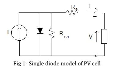
[image:1.595.338.545.209.320.2]Solar cells are the basic components of PV panels. A solar cell is basically a p-n junction which is made up of two different layers of silicon doped with a small amount of impurity. Mostly they are made of Silicon. Solar cells work on the principle of photoelectric effect according to which some semiconductors can convert electromagnetic radiation directly into electrical current. The charged particles generated by the incident radiation are separated conveniently to create an electrical current by an appropriate design of the structure of the solar cell.
Fig 1- Single diode model of PV cell
In the basic diode model of PV cell, there is a current source (I) along with a diode and series resistance (Rs). The shunt resistance (RSH) in parallel has very high value and has a negligible effect, hence can be neglected.
The output current from the photovoltaic array is-
I= Isc – Id
(1)
Id= Io (e
qVd/kT- 1)
(2)
The final expression of the current after applying
approximations to (1) & (2) is:
I = ISC - I0 [exp {q (V+IRS)/nkT}-1] (3)
Where
Io=reverse saturation current of the diode, q=electron charge,
Vd =voltage across the diode,
K=Boltzmann constant (1.38 * 10-19 J/K) T=junction temperature in Kelvin (K) n=diode ideality factor
© 2017, IRJET | Impact Factor value: 5.181 | ISO 9001:2008 Certified Journal
| Page 1716
Figure 2: I-V and P-V Characteristics Curve1.2 MPPT Requirement
[image:2.595.315.542.275.512.2]The main aim in MPPT is to control the duty ratio (D) of the converter used. In the source side we use a convertor that is connected to a solar panel in order to enhance the output voltage and by changing the duty cycle of the converter appropriately the source impedance can be matched with the load impedance.
Fig. 3. General scheme of a PV with an MPPT system.
2. DIFFERENT MPPT TECHNIQUES
2.1 Perturb & Observe
In P and O method, we use only one sensor hence it is easy to implement. Voltage sensor used senses the PV array voltage and so the cost of implementation is less. The time complexity of this algorithm is very less but on reaching very close to the MPP it keeps on perturbing on both the directions. But we can set some error limit as perturbations occurs near MPP. But this method doesn’t consider change in irradiation level due to perturbation and hence calculates the wrong MPP. To avoid this problem we can use incremental conductance method.
Fig. 4. Flowchart of P&O method.
2.2 Incremental conductance
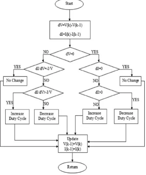
After P&O, InC is commonly used for solar PV MPPT. The incremental conductance method is based on the fact that the slope of the P vs. V (I) of the PV module is zero at the MPP, positive (negative) on the left of it and negative (positive) on the right.
dP/dV > 0 left side of the curve dP/dV < 0 right side of the curve dP/dV =0 peak of the curve
The above expressions can be expressed as:
(4)
[image:2.595.55.270.533.723.2]© 2017, IRJET | Impact Factor value: 5.181 | ISO 9001:2008 Certified Journal
| Page 1717
, At MPP, Left of MPP
, Right of MPP
[image:3.595.44.281.226.510.2]The operating point tracks MPP by comparing the immediate conductance (I/V) to the Incremental Conductance (ΔI/ΔV).
Fig. 5. Flowchart for incremental conductance method
2.3 Fractional Open Circuit Voltage
This method uses the approximately linear relationship between the MPP voltage (VMPP) and the open circuit voltage (VOC), which varies with the irradiance and temperature.
V
MPP≈ k
VOC
(5)
Where, k is a constant and depends on the array characteristics and it must be determined for different levels of irradiance. It’s value varies between 0.71 and 0.78. To measure, the system is shut down for short time which causes momentarily power loss. This analysis gives approximate value of VMPP.
2.4 Fractional Short Circuit Current
It is same as fraction open circuit, but here the relationship is between MPP current (IMPP) and short circuit current (ISC) for varying atmospheric conditions.
I
MPP≈ k’
ISC
(6)
The coefficient of proportionality k’ is obtained according to each PV array. It’s value varies between 0.78 and 0.92.To measure ISC, an additional switch to power converter is required to periodically short the PV array.
2.5 Fuzzy Logic Control
This method can deal with imprecise inputs and does not need an accurate mathematical model and can handle nonlinearity. The fuzzy logic control generally use microcontrollers. The fuzzy logic works in three stages: fuzzification, inference system and defuzzification. Fuzzification is the process of transforming crisp inputs into linguistic variables based on the degree of membership to certain sets. Membership functions are used to associate a grade to each linguistic term. The number of membership functions used depends on the accuracy of the controller, but it usually varies between 5 and 7. In second stage rule based table is designed based on some rules which associates the fuzzy output to the fuzzy inputs based on the power converter used and on the knowledge of the user.The last stage of the fuzzy logic control is the defuzzification. In the defuzzification stage the output is converted from a linguistic variable to crisp once again using membership functions.
[image:3.595.311.550.491.616.2]In the below figure, seven fuzzy levels are used: NB (Negative Big), NM (Negative Medium), NS (Negative Small), ZE (Zero), PS (Positive Small), PM (Positive Medium) and PB (Positive Big). The values a, b and c are based on the range values of the numerical variable.
Figure 6- Membership function
The inputs of the fuzzy controller are usually an error, E, and the change in the error, ∆E. The error is usually chosen as ∆P/∆V because it is zero at the MPP. Then E and ∆E are defined as follows:
© 2017, IRJET | Impact Factor value: 5.181 | ISO 9001:2008 Certified Journal
| Page 1718
Table 1- Rule based table for Fuzzy logic MPPTE\∆E NB NM NS ZE PS PM PB
NB
NB NB NB NB NM NS ZE
NM
NB NB NB NM NS ZE PS
NS
NB NB NM NS ZE PS PM
ZE
NB NM NS ZE PS
PM PB
PS
NM NS ZE PS
PM PB PB
PM
NS ZE PS
PM PB PB PB
PB
ZE PS
PM PB PB PB PB
The output of the fuzzy logic converter is usually a change in the duty ratio of the converter, ∆D, or a change in the reference voltage of DC link ∆V.
2.6 Neural Network
[image:4.595.62.268.378.532.2]Neural network and fuzzy logic comes under Soft Computing. The logic of neural network is motivated by the sophisticated functionality of human brain where hundreds of billions of interconnected neurons process information in parallel. The simplest example of a Neural Network has three layers called the input layer, hidden layer and output layer, as shown in Figure-
Figure 7- Neural Network
More complicated NN’s can be built adding more hidden layers depending on user knowledge. The input variables can be parameters of the PV array such as VOC and ISC, atmospheric data as irradiation and temperature or a combination of these. The output is usually one or more reference signals like the duty cycle or the DC-link reference voltage. The performance of the NN depends on the functions used by the hidden layer and how well the neural network has been trained. In Figure the weight between the nodes i and j is labelled as wij. The weights are adjusted in the training process. Foe this, data is recorded for a period of time, so that the MPP can be tracked accurately.
The main disadvantage of this MPPT technique is that the data needed for the training process has to be acquired for every PV array and location, as the characteristics of the PV array vary depending on the model and the atmospheric conditions depend on the location. These characteristics also
change with time, so the neural network has to be periodically trained.
2.7 Particle Swarm Optimization
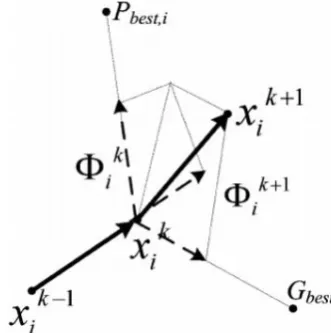
This technique is one of the highly potential technique among various evolutionary algorithms because of its simple structure, fast computation ability and easy implementation. PSO is based on the behaviour of bird groups and is a population based stochastic search method. The PSO algorithm maintains a swarm (group) of individuals (called particles), where each particle represents a candidate solution. Each particle tries to compete with the success of neighbouring particles and its own attained success. Thus the position of each particle depends on the best particle in a neighbourhood (Pb) and on the best solution (Gb) establish by all the particles in the complete population. The position of a particle (Xi) is adjusted is by using Eq (8)-
(9)
Where ∅i represents the step size of velocity component.is calculated using Eq. (9), where k1 and k2 are the acceleration coefficients, w is the inertia weight,, r1, r2 lies between 0 and 1, Pb is the best position of particle i, and Gb is the best position of the particles in the complete population.
[image:4.595.346.512.465.632.2](10)
Figure 8- Movement of particles in optimization process
© 2017, IRJET | Impact Factor value: 5.181 | ISO 9001:2008 Certified Journal
| Page 1719
Table 2: Comparison of MPPT techniques according to several parametersSr. No. MPPT technique Convergence speed Implement -ation complexity Periodic
tuning parameters Sensed
Efficiency (%) Analog or Digital Control True MPPT
Cost Control Strategy
Stability
1 Perturb & observe
Varies Low No Voltage,
Current
Medium Both Yes Moderate Sampling Not Stable
2 Incremental
conductance Varies Medium No Voltage, current
Medium Digital Yes Moderate Sampling Stable
3 Fractional Voc
Medium Low Yes Voltage Low Both No Cheap Indirect Not
Stable
4 Fractional Isc
Medium Medium Yes Current Low Both No Cheap Indirect Not
Stable
5 Fuzzy logic control
Fast High No Varies Very High Digital Yes Expensive Probabilistic Very stable
6 Neural network
Fast High No Varies Very High Digital Yes Expensive Probabilistic Very Stable
7 Particle Swarm Optimization
Fast Medium No Varies High Digital Yes Expensive Probabilistic Very Stable
3. CONCLUSIONS
From many years researchers and scientists are working on renewable energy sources. MPPT is the technique for increasing the output efficiency and mainly used for solar system and play vital role in electrical energy generation. In this study, general classification and descriptions of the most widely used seven MPPT techniques are analysed and compared to point out the advantages and drawbacks of various MPPT methods. This paper is helpful for selecting a MPPT technique depending upon various constraints as given in the table. In practice, the most widely used techniques are P&O and IC due to their simple structures and low cost. Recently, the software-based artificial intelligent techniques such as FL and ANN are growing in MPTT applications.
REFERENCES
[1] Mohammed Aslam Husain et al, “Comparative assessment of maximum power point tracking procedures for photovoltaic systems”, Energy & Environment, 2016
[2] Nevzat Onat, “Recent Developments inMaximumPower Point Tracking Technologies for Photovoltaic Systems”, International Journal of Photoenergy, 2010 [3] Nabil Karamia, Nazih Moubayed, Rachid Outbib, “General review and classification of different MPPT
Techniques”, Renewable and Sustainable Energy Reviws- Elsevier, 2017
[4] Ratna Ika Putri et al “Maximum power point tracking for photovoltaic using incremental conductance method”, Energy Procedia, April 2015, Volume 68 [5] Kashif Ishaque et al “The performance of perturb and
observe and incremental conductance maximum power point tracking method under dynamic weather conditions”, Applied Energy, 15 April 2014, Volume 119
[6] Satyananda Sarangi, “Maximum Power Point Tracking (MPPT) –A Review on Innovative Algorithms”, IJAREEIE, 2015
[7] Puneet Joshia & Sudha Arora, “Maximum power point tracking methodologies for solar PV systems – A review”, Renewable and Sustainable Energy Reviews, 2016
[8] M. A. G. de Brito, L. Galotto, L. P. Sampaio, G. de Azevedo e Melo, and C. A. Canesin, “Evaluation of the main MPPT techniques for photovoltaic applications” IEEE Transactions on Industrial Electronics, vol. 60, no. 3, pp. 1156–1167, 2013
[9] B. Subudhi and R. Pradhan, “A comparative study on maximum power point tracking techniques for photovoltaic power systems,” IEEE Transactions on Sustainable Energy, vol. 4, no. 1, pp. 89–98, 2013
[10] S. Saravanan, Ramesh Babu N., “Maximum power point
© 2017, IRJET | Impact Factor value: 5.181 | ISO 9001:2008 Certified Journal
| Page 1720
[11] Reisi AR, Moradi MH, Jamasb S., “Classification and
comparison of maximum power point tracking techniques for photovoltaic system:a review”, Renew Sustain EnergyRev2013;19:433–43
[12] Subudhi Bidyadhar, Pradhan Raseswari, “A
comparative study on maximum power point tracking techniques for photovoltaic power systems”, IEEE Trans Sustain Energy2013;4(1):89–98
[13] J. Surya Kumari, Ch. Sai Babu; “Comparison Of
Maximum Power Point Tracking Algorithms For Photovoltaic System”, International Journal of Advances in Engineering & Technology, Nov 2011
[14] Nasir Hussein Selman , Jawad Radhi Mahmood “
Comparison Between Perturb & Observe, Incremental Conductance and Fuzzy LogicMPPT Techniques at Different Weather Conditions” International Journal of Innovative Research in Science,Engineering and Technology;Vol. 5, Issue 7, July 2016
[15] Huiying Zheng ,Shuhui Li ,Ke Bao ,Dong Zhang, ”
Comparative study of maximum power point tracking control strategies for solar PV systems,” Transmission and Distribution Conference and Exposition (T&D), 2012 IEEE PES
[16] Nasir Hussein Selman , Jawad Radhi Mahmood
“Comparison Between Perturb & Observe, Incremental Conductance and Fuzzy LogicMPPT Techniques at Different Weather Conditions”, International Journal of Innovative Research in Science,Engineering and Technology;Vol. 5, Issue 7, July 2016
[17] Loredana Cristaldi, Marco Faifer, Christian Laurano,
Roberto Ottoboni, Sergio Toscani; Experimental Comparison of MPPT Algorithms
[18] Tajuddin,M.F.N.,Ayob,S.M.,Salam,Z.,Saad,M.S.,
“Evolutionary based maximum power point tracking technique using differential evolution algorithm”, Elsevier Energy and Building, Vol. 67, pp. 245 – 252, December 2013.
[19] Ishaque,K., Salam, Z., “A Deterministic Particle Swarm
Optimization Maximum Power Point Tracker for Photovoltaic System Under Partial Shading Condition”, IEEE.
[20] Dahmane,M.,Bosche,J.,EI-Hajjaji,A., Pierre,X., “MPPT for
Photovoltaic Conversion Systems Using Genetic Algorithm and Robust Control”, American Control Conference (ACC), 2013.
[21] Elgendy,M.A.,Zahawi,B.,Atkinson,D.J., “Assessment of