IceCube and ANTARES

IceCube and ANTARES

Jürgen Brunner1,a

1_{Centre de Physique de Particule de Marseille}

Abstract. IceCube and ANTARES are neutrino detectors sensitive to energies from 20 GeV up to PeV. Both

detectors have been completed and take data. Several years of data have been already analysed including periods with the partly assembled detectors. The primary goal of these two neutrino telescopes is the observation of astrophysical sources of neutrinos. Results from searches for such neutrinos with different strategies will be presented as well as measurements of atmospheric neutrinos which are an irreducible background for such searches, but they are an interesting study object by themselves.

1 Introduction

More than one hundred years after the first observations of cosmic rays, and in spite of the impressive amount of data that have in the meantime been collected, many of the problems connected with their origin and propaga-tion remain unsolved. It is a common, but poorly sup-ported, belief that they must originate from catastrophic events which take place in our as well as in other Galaxies. Events such as Supernova explosions, Active Galactic Nu-clei, Quasars and Micro Quasars, which are likely sources of high energy cosmic rays and gamma rays, could be in-tense neutrino sources as well. The measurement of the arrival direction and energy of such neutrinos, that would clarify the production mechanisms of high energy hadrons and gammas, requires very massive targets, of sizes far beyond those of present, conventional underground detec-tors. A possible solution, suggested over 20 years ago, is the use of water or ice as a Cherenkov target-detector. The prove of this concept has been performed in lake Baikal with the unambiguous detection of atmospheric neutri-nos in the NT-96 detector [1]. Today two large detectors, ANTARES in the Mediterranean Sea and IceCube at the South pole take data and produce physics results. These two projects will be presented in the following.

2 ANTARES

A detailed description of the ANTARES detector can be found in [2]. The detector consists of 12 lines, equipped with photosensors, and a junction box which distributes the power and clock synchronization signals to the lines and collects the data. The junction box is connected to the shore by a 42 km electro-optical cable. The length of the detection lines is 450 m, of which the lowest 100 m are not instrumented. Their horizontal separation is about 65 m

a_{e-mail: [email protected]}

and they are arranged to form a regular octagon on the sea floor. They are connected to the junction box with the help of a submarine using wet-mateable connectors. Each line comprises 25 storeys each separated by a vertical distance of 14.5 m. The lines are kept taut by a buoy at the top of the line and an anchor on the seabed. The movement of the line elements due to the sea currents is continuously mea-sured by an acoustic calibration system with an accuracy of 10 cm [3].

Each storey contains three 45◦ downward-looking 10” photomultiplier tubes (PMT) inside pressure resis-tant glass spheres - the optical modules [4]. Some of the storeys contain supplementary calibration equipment such as acoustic hydrophones or optical beacons [5].

The signals of each photomultiplier are readout by two ASICs. The charges and arrival times of the PMT sig-nals are digitised and stored for transfer to the shore sta-tion [6]. The time stamps are synchronised by a clock signal which is sent at regular intervals from the shore to all electronic cards. The overall time calibration is better than 0.5 ns [7]. Therefore the time resolution of the signal pulses is limited by the transit time spread of the photo-multipliers (σ ∼1.3 ns) [8] and by chromatic dispersion for distant light sources. All data are sent to the shore sta-tion. With the observed optical background rate of 70 kHz per PMT at the single photon level this produces a data flow of several Gbit/s to the shore. In the shore station a PC farm performs a data filtering to reduce the data rate by at least a factor of 100 [9]. Several trigger algorithms are applied depending on the requested physics channel and on the observed optical noise.

The first detection line had been installed in 2006. From March to December 2007 ANTARES operated in a 5-line configuration, followed by several months of op-eration with 10 installed detector lines. The detector con-struction was completed in May 2008.

C

Owned by the authors, published by EDP Sciences, 2013

This is an Open Access article distributed under the terms of the Creative Commons Attribution License 2 0 , which . permits unrestricted use, distributi and reproduction in any medium, provided the original work is properly cited.

3 IceCube

The IceCube detector [10] consists of 5,160 digital optical modules. Each of them contains a photomultiplier tube (identical to ANTARES), supporting hardware and elec-tronics inside a pressure glass sphere. These optical mod-ules are arranged on 86 strings frozen into the antarctic ice at depths from 1450 m to 2450 m with a spacing of 120 m between adjacent strings, instrumenting one cubic kilome-ter. Optical properties of South Pole ice are depth depen-dent. Typical optical absorption lengths are 100-140 m and typical optical effective scattering lengths are 25-35 m. The latter limits the time resolution of the signal pulses from Cherenkov light to about 6 nsec, degrading thereby the ultimate angular resolution reachable from muon track reconstruction. Unlike sea water Antarctic ice has a low concentration in radioactive isotopes. In particular 40_K, abundant in salty sea water, is absent in ice. Further, no light-producing biological activity occurs. Therefore, the observed optical background rate at the single photon level is only 500 Hz per PMT in IceCube.

Beginning with the installation of the first string in 2005, IceCube has been operated in approximately year-long data taking seasons. During the antarctic summer seasons in December and January new strings had been de-ployed at a pace of about 20 strings per year. IceCube con-struction was finished in December 2010. From May 2008 to April 2009 IceCube operated with 40 installed strings, the so-called IC40 configuration. From May 2009 to April 2010 59 strings had been active (IC59). The results which will be presented in the following have been obtained from analysing these two data-taking periods.

4 Neutrino Interactions: the cascade and

the muon channel

Neutrino interactions in the vicinity of the detector lead to two distinct signatures which are exploited in independent analyses. The charged current interaction of muon neutri-nos

νµ(¯νµ)+N→µ∓+X (1)

and the charged current interaction of tau neutrinos with a subsequent muonic decay

ντ(¯ντ)+N→ τ∓+X (2)

τ∓→µ∓+ν¯µ(νµ)+ντ(¯ντ) (3)

result both in a long muon track. At TeV and even more at PeV energies these muons have a range of several km in water or ice, largely exceeding the size of the detec-tors. The neutrino interaction vertex and the accompany-ing hadronic shower are outside the fiducial volume most of the time. The track signature yields a good angular res-olution and ensures a clean separation of an upward going neutrino signal from the background of downward going atmospheric muons. The muon energy at the detector is deduced from the energy loss dE/dx which is related to the “brightness" of the track in the detector. As the energy loss is mostly stochastic at TeV/PeV energies, the muon

energy can only be estimated with a precision of about a factor two. The calculation of the related neutrino energy depends on the assumed neutrino flux because the muon track has to be extrapolated upstream the detector to the neutrino vertex.

All other neutrino interactions as neutral current reac-tions

νx(¯νx)+N→νx(¯νx)+X (4)

electron neutrino charged current interactions

νe(¯νe)+N→e∓+X (5)

and charged current interactions of tau neutrinos with a subsequent non-muonic decay

ντ(¯ντ)+N→ τ∓+X (6)

τ∓→ντ(¯ντ)+X (7)

lead to a so-called cascade signature with the exception of tau neutrino charged current interactions at energies above 10 PeV which would yield two distinct cascades, one at the neutrino interaction vertex and a second one at the tau decay point. This special case is not considered in the fol-lowing.

As a result of these neutrino interactions one obtains a hadronic and, depending on the channel, also an electro-magnetic shower. They are very narrow and have a lon-gitudinal extension of at most a few tens of meters. Due to the large spacing of adjacent detector elements in the coarsely equipped neutrino telescopes it is impossible to distinguish electromagnetic from hadronic showers. The observable signature in the detector is in all cases an iso-lated “cascade". Due to its small extension the angular resolution is worse here than for the track signature. This compromises the up/down separation. The main back-ground for the cascade search comes from bright elec-tromagnetic showers (e.g. due to bremsstrahlung) which accompany downward going atmospheric muons. The en-ergy resolution for cascades can be better than for the track channel. All particles but the escaping neutrinos are seen in the detector and the brightness of the events correlates directly to the cascade energy which in turn is closely re-lated to the neutrino energy. When using containment con-ditions for the neutrino vertex the power of the background rejection as well as the energy resolution can be further improved.

Whereas the effective volume for the cascade channel is close to the equipped volume of the detector, it is sig-nificantly larger for the muon channel due to the very long muon range.

5 Atmospheric Neutrinos

The main sources of conventional atmospheric neutrinos are their decays

π± _→µ±_{+νµ(¯νµ) (8)}

K± _→µ±_+ν

µ(¯νµ) (9)

K± _→e±_{+νe(¯νe)+π}0_{. (10)}

The subsequent decay of the muon contributes only marginally to the multi-GeV neutrino flux as most of these muons reach the ground and they are stopped before de-caying. The primary Cosmic Rays have a non-thermal E−γ spectrum withγ ≈ 2.7. As pions and kaons propagate a certain distance through the atmosphere and lose thereby energy before decaying, the resulting neutrino spectrum is softer withγ≈3.7.

The most recent measurements of the high energy part of the atmospheric neutrino spectrum comes from the Ice-Cube collaboration [11, 12]. One year of data has been analysed in the IC40 configuration. As many as 18,000 upward goingνµcandidate events have been selected for this analysis. So far only the track signature has been ex-ploited to measure the atmospheric neutrino flux above 100 GeV. This has several reasons. Firstνµare more co-piously produced than other flavours (see Equation 8,9) and neutral current interactions have a lower cross section than charged current reactions. Further the effective vol-ume is larger for the muon track signal than for the cascade channel and finally the isolation of a clean upward going event sample is more difficult in the cascade channel, as discussed above.

Two methods have been used to extract the neutrino spectrum from the data, forward folding [11] and regular-ized unfolding [12]. Both methods give comparable re-sults and they are also consistent with different conven-tional atmospheric neutrino flux calculations [13, 14]. A distinction between these different flux predictions is not possible within the precision of the measurement. The highest energetic events can be attributed to neutrinos with energies of more than 100 TeV, which are thereby the high-est energetic neutrino interactions ever detected.

For neutrino energies above 10 TeV the decay of mesons which contain heavy quarks (c,b) starts to con-tribute to the atmospheric neutrino flux. As these mesons have typical decay lengths of only few mm, they do not lose energy before they decay and the resulting so-called prompt atmospheric neutrino spectrum follows closely the original Cosmic Ray spectrum, i.e. γ≈2.7. This should be seen as a hardening of the measured spectrum and has been searched for in one of the mentioned IceCube anal-yses [11]. The predictions for this prompt neutrino flux vary by up to a factor ten [15–19]. The largest contribu-tion is obtained in the frame of the Recombinacontribu-tion Quark Parton Model [17–19] (RQPM), a non-perturbative QCD approach. As no hardening of the neutrino spectrum is ob-served, the RQPM model from [17] can be excluded on a level of 3σin [11]. Further the model from [16] contains free parameters. When choosing these parameters to max-imize the prompt neutrino flux, this model can be excluded with 2σ. The model from [15], which predicts the lowest

prompt flux, can instead not be constrained by the current data.

6 Search for Diffuse Neutrino Fluxes

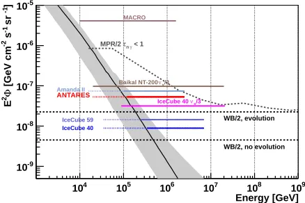
For neutrino energies larger than 10 TeV searches are per-formed for an additional, extraterrestrial component in the measured flux. This component is expected to be harder withγ ≈2.0. An upper bound for a diffuse neutrino flux from astrophysical sources has been derived by Waxman and Bahcall (W&B) [20]. Here it is assumed that the ex-tragalactic Cosmic Ray spectrum for E >1018_{eV is} pro-duced in sources where protons are magnetically confined to undergo efficiently the photoproduction reaction

p+γ→∆+→n+π+. (11)

The pions decay according to Equation 8 and produce neutrinos, whereas the neutrons escape from the accel-eration site, decay and produce the observed high ener-getic Cosmic Ray spectrum. Therefore the predicted neu-trino flux is closely related to the observed Cosmic Ray flux above E > 1018 eV and should be proportional to

E−2over several orders of magnitude. The resulting upper bound, corrected for neutrino oscillations during propaga-tion from the source to Earth (indicated by the factor “/2”) and scaled to recent measurements of the highest energetic Cosmic ray flux is shown on Figure 1. Other models try to circumvent the constraints of [20] and predict higher neutrino fluxes. One example [21], already excluded by existing limits, is also shown on Figure 1.

Energy [GeV]

4

10 ₁₀5 ₁₀6 ₁₀7 ₁₀8 ₁₀9

]

-1

sr

-1

s

-2

[GeV cm

Φ

2

E

-9

10

-8

10

-7

10

-6

10

-5

10

WB/2, evolution

WB/2, no evolution < 1

γ n τ MPR/2

ANTARES

MACRO

Amanda II

/3

x ν

Baikal NT-200

IceCube 40 IceCube 59

/3 x ν IceCube 40

Figure 1. A comparison of 90% C.L. upper limits for E−2_diffuse

neutrino fluxes and theoretical models. For details, see text.

neutrino candidates. The energy is estimated by evaluat-ing the “brightness per track length" which correlates with the muon energy loss and therefore the muon energy in the detector. Two analyses have instead exploited the cascade channel [24, 26]. As such an analysis is sensitive to all neutrino flavours, a scaling factor three (indicated by “/3” in the figure) is applied to make the resulting limits com-patible to the muon channel limits. The crucial parameter in the cascade analysis is the absolute event brightness, ex-pressed in terms of hit counts or amplitude, which is used as an energy proxy and allows to distinguish the signal from background.

The energy range of the limit lines in Figure 1 indicates the central range in which 90% of the signal events are ex-pected. For the muon channel, the lowest testable energies are at the level, where the contribution from atmospheric neutrinos becomes stronger. As this contribution is signif-icantly lower in the cascade channel (not shown in the fig-ure), the limits derived in this channel extend subsequently to lower energies.

The most recent result has been obtained by analysing 21943 events from 348 days of data taking with the IC59 setup in IceCube [27]. It is interesting to note, that the re-sulting limit is slightly worse than the limit which had been previously obtained with the smaller IC40 setup [11]. This is due to fluctuations in the high energy tail of the IC59 data set. However the size of the excess is not statistically significant.

7 Search for Neutrino Point Sources

The ultimate goal of neutrino telescopes is it to provide a sky map in neutrinos. This requires the identification of individual neutrino sources in the sky and is complemen-tary to the search for a diffuse flux, as described in the previous section. High energy neutrinos can be produced through Fermi acceleration of protons in relativistic shock waves with subsequent hadronic interactions and pion de-cays. From observation with photons such shock waves are known to exist in various objects in our own Galaxy as well as up to cosmological distances. Various mod-els for neutrino production exist [28–30]. Promising neu-trino point source candidates in our own Galaxy are Super-novae Remnants and Micro Quasars whereas the vicinity of the super-massive black holes in Active Galactic Nu-clei and Gamma Ray Bursts are prominent extragalactic candidates.

The first step in the neutrino point source search con-sists in isolating a suitable set of candidate events. For upgoing events in ANTARES and IceCube the selected events are mostly atmospheric neutrinos. For downgo-ing events, as analysed in IceCube, the candidate events are high-energetic Cosmic Ray muons. These two event classes follow an almost isotropic distribution on small an-gular scales. A neutrino point source could be identified as an accumulation of events above background around the source. To quantify the discovery potential for a given point source candidate a likelihood ratio method is used. For each event the likelihood is calculated for the hypoth-esis that it is background (i.e. has an atmospheric origin)

declination (degrees)

-80 -60 -40 -20 0 20 40 60 80

)

-1

s

-2

flux limit ( GeV cm

×

ν

2

E

-9

10

-8

10

-7

10

-6

10

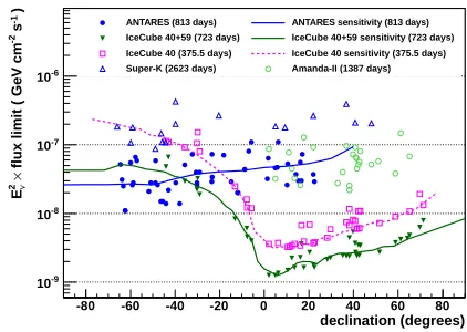
ANTARES (813 days) ANTARES sensitivity (813 days) IceCube 40+59 (723 days) IceCube 40+59 sensitivity (723 days) IceCube 40 (375.5 days) IceCube 40 sensitivity (375.5 days) Super-K (2623 days) Amanda-II (1387 days) ANTARES (813 days) ANTARES sensitivity (813 days) IceCube 40+59 (723 days) IceCube 40+59 sensitivity (723 days) IceCube 40 (375.5 days) IceCube 40 sensitivity (375.5 days) Super-K (2623 days) Amanda-II (1387 days) ANTARES (813 days) ANTARES sensitivity (813 days) IceCube 40+59 (723 days) IceCube 40+59 sensitivity (723 days) IceCube 40 (375.5 days) IceCube 40 sensitivity (375.5 days) Super-K (2623 days) Amanda-II (1387 days) ANTARES (813 days) ANTARES sensitivity (813 days) IceCube 40+59 (723 days) IceCube 40+59 sensitivity (723 days) IceCube 40 (375.5 days) IceCube 40 sensitivity (375.5 days) Super-K (2623 days) Amanda-II (1387 days)

Figure 2. A comparison of 90% C.L. upper limits for E−2

neu-trino fluxes for predefined point source searches. For details, see text.

or it is signal (i.e. comes from the source). This likelihood takes into account the angular resolution of the events and their energy. The test statistics is the ratio of the two likeli-hoods, summed over all events in the vicinity of the source candidate. The simulation of many background-only sky maps allows to determine the probability of background fluctuations.

Two methods are used to identify neutrino point sources. In the all-sky-search it is assumed that a source exists somewhere in the sky. Its position is not fixed and it is obtained as the result from a fit to the actual event distribution. When using instead a predefined source list, the source hypothesis is only tested at the positions of the most promising candidates which have been selected a

pri-ori by their potential to emit neutrinos and to be seen in the

experiment.

8 Conclusion

During the last years a wealth of new results have been published on the search for neutrino fluxes from astrophys-ical sources from both ANTARES and IceCube. Several methods are used to identify such extraterrestrial neutri-nos. The most prominent ones are the search for a high energy component to the measured diffuse neutrino flux and by point source searches either from a predefined list of candidate sites for neutrino emission or as a full sky search for a hitherto unknown point in the sky which hides a neutrino source. So far none of these analyses found any excess of events beyond the expected rate of atmospheric neutrino events. The sensitivity of the analyses is already high enough to constrain or exclude various models. For the first time fluxes below the W&B upper bound [20] are tested.

References

[1] V. Balkanov et al. [BAIKAL Coll.], In “Salt Lake City 1999, Cosmic ray”, vol. 2 (1999) 176.

[2] M. Ageron et al., [ANTARES Coll.], Nucl. Instrum.

Meth. A656 (2011) 11.

[3] S. Adrian-Martinez et al., [ANTARES Coll.], JINST

7 (2012) T08002.

[4] P. Amram et al., [ANTARES Coll.], Nucl. Instrum.

Meth. A484 (2002) 369.

[5] M. Ageron et al., [ANTARES Coll.], Nucl. Instrum.

Meth. A578 (2007) 498.

[6] J. A. Aguilar et al., [ANTARES Coll.], Nucl.

In-strum. Meth. A622 (2010) 59.

[7] J. A. Aguilar et al., [ANTARES Coll.], Astropart.

Phys. 34 (2011) 539.

[8] J. A. Aguilar et al., [ANTARES Coll.], Nucl.

In-strum. Meth. A555 (2005) 132.

[9] J. A. Aguilar et al., [ANTARES Coll.], Nucl.

In-strum. Meth. A570 (2007) 107.

[10] F. Halzen and S.R. Klein, arXiv:1007.1247.

[11] R. Abbasi et al., [IceCube Coll.], Physical Review D

84 (2011) 082001.

[12] R. Abbasi et al. [IceCube Coll.], Phys. Rev. D 83 (2011) 012001.

[13] G.D. Barr, T.K. Gaisser, P. Lipari, S. Robbins and T. Stanev, Phys. Rev. D 70 (2004) 023006.

[14] M. Honda, T. Kajita, K. Kasahara, S. Midorikawa, and T. Sanuki, Phys. Rev. D 75 (2007) 043006. [15] A. D. Martin, M. G. Ryskin, and A. M. Stasto, Acta

Phys. Pol. B 34 (2003) 3273.

[16] R. Enberg, M.H. Reno, and I. Sarcevic, Phys. Rev. D

78 (2008) 043005.

[17] E. Bugaev et al., Phys. Rev. D 58 (1998) 054001. [18] G. Fiorentini, A. Naumov, and F. L. Villante, Phys.

Lett. B 510 (2001) 173.

[19] C.G.S. Costa, Astropart. Phys. 16 (2001) 193. [20] E. Waxman and J. Bahcall, Phys. Rev. D 59 (1998)

023002-1;

J. Bahcall, E. Waxman, Phys. Rev, D 64 (2001) 023002-1.

[21] K. Mannheim, R. J. Protheroe, J. P. Rachen, Phys. Rev. D 63 (2000) 023003.

[22] M. Ambrosio et al., [MACRO Coll.], Astrop. Phys.

19 (2003) 1.

[23] A. Achterberg et al., [Amanda Coll.], Phys. Rev. D

76 (2007) 042008.

[24] A.V.Avrorin et al., [Baikal Coll.], Astronomy Letters

35 (2009) 651.

[25] J.A. Aguilar et al., [ANTARES Coll.], Phys. Lett. B

696 (2011) 16.

[26] R. Abbasi et al., [IceCube Coll.], arXiv:1111.2736 [astro-ph.HE].

[27] G.W. Sullivan et al., [IceCube Coll.], Presentation at “Neutrino 2012”, http://neu2012.kek.jp/

[28] F. Halzen and D. Hooper, Rep. Prog. Phys. 65 (2002) 1025.

[29] W. Bednarek, G.F. Burgio and T. Montaruli, New As-tron. Rev. 49 (2005) 1.

[30] F.W. Stecker, Phys. Rev. D 72 (2005) 107301. [31] E. Thrane et al., [SuperK Coll.], Astrophysical

Jour-nal 704 (2009) 503.

[32] R. Abbasi et al., [Amanda Coll.], Phys. Rev. D 79 (2009) 062001.

[33] S. Adrian-Martinez et al., [ANTARES Coll.], Astro-physical Journal 760 (2012) 53.