Data-Driven Learning of Boolean Networks and Functions by Optimal Causation
1
Entropy Principle (BoCSE)∗
2
Jie Sun†, Abd AlRahman R AlMomani‡, and Erik Bollt§ 3
4
Abstract. Boolean functions and networks are commonly used in the modeling and analysis of complex
bio-5
logical systems, and this paradigm is highly relevant in other important areas in data science and
6
decision making, such as in the medical field and in the finance industry. In a Boolean model, the
7
truth state of a variable is either 0 or 1 at a given time. Despite its apparent simplicity, Boolean
8
networks are surprisingly relevant in many areas of application such as in bioinformatics to model
9
gene expressions and interactions. In the latter case, a gene is either “on” or “off” depending on its
10
expression level. Despite the promising utility of Boolean modeling, in most practical applications
11
the Boolean network is not known. Automated learning of a Boolean network and Boolean
func-12
tions, from data, is a challenging task due in part to the large number of unknowns (including both
13
the structure of the network and the functions) to be estimated, for which a brute force approach
14
would be exponentially complex. In this paper we develop a new information theoretic methodology
15
that we show to be significantly more efficient than previous approaches. Building on the recently
16
developed optimal causation entropy principle (oCSE), that we proved can correctly infer networks
17
distinguishing between direct versus indirect connections, we develop here an efficient algorithm
18
that furthermore infers a Boolean network (including both its structure and function) based on data
19
observed from the evolving states at nodes. We call this new inference method, Boolean optimal
20
causation entropy (BoCSE), which we will show that our method is both computationally efficient
21
and also resilient to noise. Furthermore, it allows for selection of a set of features that best explains
22
the process, a statement that can be described as a networked Boolean function reduced order model.
23
We highlight our method to the feature selection in several real-world examples: (1) diagnosis of
24
urinary diseases, (2) Cardiac SPECT diagnosis, (3) informative positions in the game Tic-Tac-Toe,
25
and (4) risk causality analysis of loans in default status. Our proposed method is effective and
26
efficient in all examples.
27
Key words. Boolean function, Boolean network, causal network inference, information flow, entropy,
quantita-28
tive biology
29
AMS subject classifications. 62M86, 94A17, 37N99
30
1. Introduction. In this paper we consider an important problem in data science and
31
complex systems, that is the identification of the hidden structure and dynamics of a complex
32
system from data. Our focus is on binary (Boolean) data, which commonly appears in many
33
application domains. For example, in quantitative biology, Boolean data often comes from
34
gene expression profiles where the observed state of a gene is classified or thresholded to either
35
∗
Submitted to the editors DATE.
Funding: This work was funded in part by the U.S. Army Research Office grant W911NF-16-1-0081 and the Simons Foundation grant 318812.
†
Department of Mathematics, Clarkson University, Potsdam, NY 13699, and Clarkson Center for Complex Systems Science, Potsdam, NY 13699
‡
Clarkson Center for Complex Systems Science, Potsdam, NY 13699, and Department of Electrical and Computer Engineering, Clarkson University, Potsdam, NY 13699
§
Clarkson Center for Complex Systems Science, Potsdam, NY 13699, and Department of Electrical and Computer Engineering, Clarkson University, Potsdam, NY 13699
“on” (high expression level) or “off” (low to no expression level). In such an application, it
36
is a central problem to understand the relation between different gene expressions, and how
37
they might impact phenotypes such as occurrence of particular diseases. The interconnections
38
among genes can be thought of as forming a Boolean network, via particular sets of Boolean
39
functions that govern the dynamics of such a network. The use of Boolean networks has many
40
applications, such as for the modeling of plant-pollinator dynamics [4], yeast cell cycles [17,8],
41
pharmacology networks [14], tuberculosis latency [12], regulation of bacteria [20], biochemical
42
networks [13], immune interactions [29], signaling networks [32], gut microbiome [25], drug
43
targeting [31], drug synergies [10], floral organ determination [2], gene interactions [1], and
44
host-pathogen interactions [23]. In general, the problem of learning Boolean functions and
45
Boolean networks from observational data in a complex system is an important problem to
46
explain the switching relationships in these and many problems in science and engineering.
47
To date, many methods have been proposed to tackle the Boolean inference problem [18,
48
16,9,21,30,3,19]. Notably, REVEAL (reverse engineering algorithm for inference of genetic
49
network architectures), which was initially developed by Liang, Fuhrman and Somogyi in
50
1998 [18] has been extremely popular. REVEAL blends ideas from computational causality
51
inference with information theory, and has been successfully applied in many different contexts.
52
However, a main limitation of REVEAL is its combinatorial nature and thus suffers from
53
high computational complexity cost, making it effectively infeasible for larger networks. The
54
key challenge in Boolean inference are due to two main factors: (1) The system of interest
55
is typically large, containing hundreds, if not thousands and more, components; (2) The
56
amount of data available is generally not sufficient for straightforward reconstruction of the
57
joint probability distribution. In this paper, we propose that information flow built upon
58
causation entropy (CSE) for identifying direct versus indirect influences, [26, 27], using the
59
optimal causation entropy principle (oCSE) [28] is well suited to develop a class of algorithms
60
that furthermore enable computationally efficient and accurate reconstruction of Boolean
61
networks and functions, despite noise and other sampling imperfections. Instead of relying on
62
a combinatorial search, our method iteratively and greedily finds relevant causal nodes and
63
edges and the best Boolean function that utilizes them, and thus is computationally efficient.
64
We validate the effectiveness of our new approach that here we call, Boolean optimal causation
65
entropy (BoCSE) using data from several real-world examples, including for the diagnosis of
66
urinary diseases, Cardiac SPECT diagnosis, Tic-Tac-Toe, and risk causality analysis of loans
67
in default status
68
This the paper is organized as follows. In Section 2 we review some basic concepts that
69
define structure and function of Boolean networks and the problem of learning these from data.
70
In Section 3 we present BoCSE as an information-theoretic approach together with a greedy
71
search algorithm with agglomeration and rejection stages, for learning a Boolean network. In
72
Section 4 we evaluate the proposed method on synthetic data as well as data from real-world
73
examples, including those for automated diagnosis, game playing, and determination of causal
74
factors in loan defaults. Finally, we conclude and discuss future work in Section 5, leaving
75
more details on the basics of information theory in the Appendix.
76
2. The Problem of Learning a Boolean Network from Observational Data.
2.1. Boolean Function, Boolean Table, and Boolean Network. A function of the form
78
(1) f :D→B, whereB={0,1},
79
is called a Boolean function, whereD⊂Bkandk∈Nis the arity of the function. For ank-ary
80
Boolean function, there are 2kpossible input patterns, the output of each is either 0 or 1. The
81
number of distinct k-ary Boolean functions is 22k, a number that clearly becomes extremely
82
large, extremely quickly, with respect to increasing k. Consider for example, 223 = 256,
83
225 ≈4.295×10⁹, and 228 ≈1.158×1077(comparable to the number of atoms in the universe,
84
which is estimated to be between 1078 and 1082). This underlies the practical impossibility of
85
approaching a Boolean function learning problem by brute force exhaustive search.
86
Each Boolean function can be represented by a truth table, called a Boolean table. The
87
table identifies, for each input pattern, the output of the function. An example Boolean
88
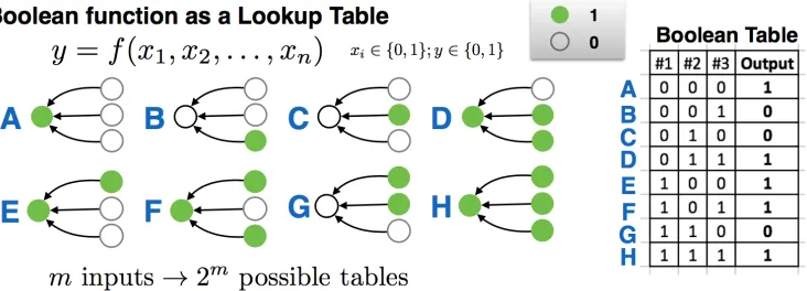
functiony=f(x1, x2, x3) together with its corresponding Boolean table are shown in Fig.1.
Figure 1. A Boolean function can be uniquely identified by a truth table, called a Boolean table. For a k-ary Boolean function, the table has2krows, andk+ 1columns. For each row, the firstk entries correspond to a particular input binary string (e.g.,(0,1,0)), and the last entry represents the output of the function.
89
A Boolean function is useful to model a system that has multiple binary inputs and a
90
single binary output. More generally, a system can have multiple outputs, in which case
91
multiple Boolean functions are needed, each capturing the relation between an output
vari-92
able and the set of input variables. The collection of these individual functions constitute a
93
Boolean network. Formally, a Boolean network is characterized by a triplet of sets, denoted
94
as G = (V;E;F), where (V;E) represents a graph that encodes the structure of the
net-95
work: V(G) = {1,2, . . . , n} is the set of nodes, and E(G) ⊂ V ×V is the set of directed
96
edges (possibly including self-loops). The functional rules of the network are encoded in
97
F(G) = (f1, f2, . . . , fn), which is an ordered list of Boolean functions. For each nodeiin the 98
network, we represent its set of directed neighborsby Ni ={j: (i, j)∈E} and the degree of
99
node ias the cardinality of Ni, denoted as ki =|Ni|. Thus, fi :Bki → Bis a ki-ary Boolean
100
function that represents the dependence of the state of node i on the state of its directed
101
neighbors. Note that alternatively the dependence patterns of a Boolean network can also be
represented by an adjacency matrixA= [Aij]n×n, where:
103
(2) Aij =
(
1, ifj∈ Ni;
0, otherwise.
104
Thus, the adjacency matrix A encodes the structure of a Boolean network, although not the
105
functional rules.
106
2.2. Stochastic Boolean Function and Stochastic Boolean Network. In practice, the
107
states and dynamics of a system are almost always subject to noise. Therefore, it is important
108
to incorporate randomness and stochasticity into a Boolean network. To do so, we first extend
109
the Boolean function concept from the deterministic definition to a stochastic generalization,
110
defining astochastic Boolean function (SBF) as
111
(3) g(x) =f(x)⊕ξ,
112
wherefis a (deterministic) Boolean function andξis a Bernoulli random variable that controls
113
the level of randomness of the function. In this model, the function contains a deterministic
114
part, given by the Boolean function f(x); the actual output of the function g(x) is given by
115
the output off(x) subject to a certain probably of being switched.
116
Following the notion of a stochastic Boolean function, we now define astochastic Boolean 117
networkas a quadruple of sets,G= (V;E;F;q), where the triplet of sets (V;E;F) represents
118
a (deterministic) Boolean network, and the vector q = [q1, . . . , qn]> ∈ [0,1]n represents the 119
level of noise, each as a random variable each withqi quantifying the probability of switching
120
the output state at node i, a scalar parameter describing the Bernoulli random variableξi ∼
121
Bernoulli(qi).
122
2.3. Data from Boolean Functions and Boolean Networks. We start by discussing
sev-123
eral forms of data that commonly appear in application problems. These include: (a)
Input-124
output data from a single Boolean function; (b) Input-output data from a Boolean network,
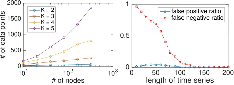
125
which can be regarded as a generalization of (a); (c) Time series data from a Boolean network.
126
In each one of these scenarios, the data can either be directly represented or rearranged into
127
a set of input-output pairs
128
(4) {(x(t),y(t)) :t= 1, . . . , T},
129
where,
130
x(t) = [x1(t), . . . , xn(t)]> ∈ Bn={0,1}n, and, 131
y(t) = [y1(t), . . . , y`(t)]>∈ B` ={0,1}`, (5)
132
are both vectors of Boolean states. We expand our discussion on this below.
133
(a) Input-output data from a single Boolean function. For a Boolean function (either
134
deterministic or stochastic), if observations or measurements are made about its inputs and
135
outputs, such data can be represented in the form of (4) where y(t) is a scalar (i.e., `= 1).
Here each pair (x(t),y(t)) represents the observed input string ofkbits, encoded inx(t), and
137
the corresponding outputy(t). The ordering of the input-output pairs is arbitrary.
138
(b) Input-output data from a Boolean network. For a (deterministic or stochastic)
139
Boolean network of nnodes, input-output data of the network comes in the form similar to
140
that of a single Boolean function, except that each output itself it no longer a single bit,
141
but instead multiple bits representing the state of all the nodes in the network. Thus, the
142
dimensionality of x(t) andy(t) are both equal ton, that is,`=nin the general form of (4).
143
The ordering of input-output pairs is arbitrary.
144
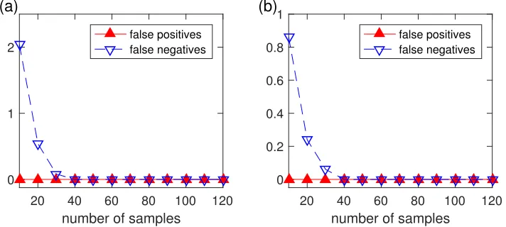
(c) Time series data from a Boolean network. For a time series observed on a Boolean
145
network ofnnodes, we can represent such data using a sequence of Boolean vectors (x(t))Tt=0,
146
where x(t) = [x1(t), . . . , xn(t)]> ∈ Bn represents the state of the entire network at time t.
147
The pair (x(t−1),x(t)) can be described as an input-output data pair from the underlying
148
Boolean network. For this matter, time series data from a Boolean network can also be put
149
into the input-output data form (4) with the additional constraint that
150
(6) y(t) =x(t+ 1) for every t= 1, . . . , T −1.
151
Here, unlike the case of input-output data as in (a) and (b), the temporal ordering in the time
152
series data is unique and should not be (arbitrarily) changed.
153
To summarize, in these three commonly encountered scenarios as we discussed above,
154
observational data from a Boolean network can be represented as input-output pairs as in (4).
155
When the network contains only one node it is really just a Boolean function and thus eachy(t)
156
is a scalar; on the other hand, when the data comes from time series then eachy(t) =x(t−1)
157
and the temporal ordering of the data becomes fixed.
158
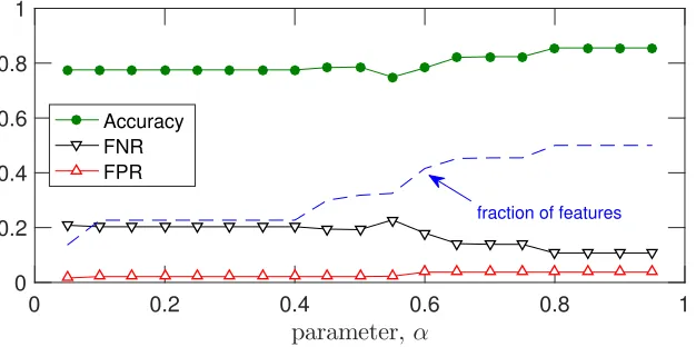
2.4. The Problem of Learning the Structure and Function of a Boolean Network.
159
Given Boolean data in the standardized form (4), we interpret data as samples of a multivariate
160
conditional probability distribution
161
p(y|x) = Prob(Y(t) =y|X(t) =x) (7)
162
= k
Y
i=1
Prob(Yi(t) =yi|X(t) =x) = k
Y
i=1
p(yi|x), (8)
163
wherex∈ Bk and y∈ B`, and thus
164
(9) p(yi|x) =p(yi|x1, . . . , xn).
165
The problem of reconstructing, or learning the Boolean network then is, canp(yi|x) be
maxi-166
mally reduced to a lower dimensional distribution. That is, does there exist a smallest (sub)set
167
of indices,
168
(10) Si⊂ {1, . . . , `}, such thatp(yi|x) =p(yi|xSi)? 169
Once we have identified, for each i, this set of nodes Si, they together constitute a network,
170
where a directed link j → i corresponds to having j ∈ Si. Furthermore, to identify such a
171
subset of explaining variables that closely approximates this conditional equality statement
172
represents a simplified or reduced order presentation of the process.
3. BoCSE for Data-Driven Learning of the Structure and Function of Boolean
Net-174
works. In this section we develop a computational framework to reconstruct both thestructure 175
andfunctionof a Boolean network from observational data. We start with the reconstruction
176
of a minimally sufficient Boolean function from input-output data. This method is repeated
177
to find the neighbor set and function for each node, and as a result reconstructs the whole
178
network.
179
3.1. Reconstruction of a Minimally Sufficient Boolean function. Given a set of
input-180
output pairs{x(t), y(t)}, (herey(t) is a single bit), we want to find a minimal Boolean function
181
that is sufficient in representing the data. To quantify the complexity of the Boolean function,
182
we state the following information-theoretic criterion
183
(11)
(
minK⊂[n]|K|,
s.t. I(X(K);Y) = maxK∈[n]I(X(K);Y) 184
Here,
185
[n={1,2, . . . , n},
186
K={k1, . . . , k`} is a subset of [n],
187
Y = [y(1), . . . , y(t)]>, and
188
X(K)= [X(K)]T×` where [X(K)]tj =X(t)kj.
(12)
189
The symbol I denotes mutual information, that is, I(X(K);Y) is the mutual information
190
betweenX(K) andY.
191
At a glance, solving this combinatorial problem seems to be computationally complex.
192
However, in our previous work [28] we developed an oCSE algorithm that can find K
effi-193
ciently, and we proved in [28] that it correctly infers the underlying network as it is able to
194
distinguish direct versus indirect connections correctly. Here we will further develop the
con-195
cept to also learn the associated Boolean functions on the networks, that here we call BoCSE.
196
Although various extensions of the oCSE algorithm are possible, some may even yield better
197
results in certain scenarios. We focus here on the most basic version of our otherwise greedy
198
search algorithm that consists of only two stages, a forward selection stage and a backward
199
elimination stage.
200
• Forward selection. We initialize the solution set Kf = ∅, and, in each iteration, we
201
choose an elementk that satisfies the following conditions
202
(13)
(
maxjI(Xj;Y|X(Kf))>0,
k= arg maxjI(Xj;Y|X(Kf)). 203
If such a kexists, then we append it to the set Kf and proceed to the next iteration;
204
otherwise, when no such kexists, the forward selection is terminated.
205
• Backward elimination. Start withKb =Kf, in each step of backward elimination, we
206
select an element kthat satisfy the following
207
(14) k= arg min
j∈Kb
Such kalways exists since Kb is a finite set. Then, if
209
(15) I(Xk;Y|X(Kb/{k})) = 0,
210
we removek fromKb and repeat; otherwise, the algorithm terminates.
211
The result of the algorithm is a set Kb ={k1, . . . , k`}, which is an estimate of the index set
212
of the minimal Boolean function that fits data. Finally, given such a setKb, we construct the
213
corresponding Boolean function by estimating the best output (0 or 1) for each unique input
214
pattern available from the data. Symbolically, for eachx0 ∈B`, we define the set
215
(16) TKb(x0) ={t:x
(Kb)(t) =x 0}, 216
and define
217
(17) g(x0) =
P
t∈TKb(x0)y(t)
|TKb(x0)|
∈[0,1].
218
Then, we obtainf :B`→Busing the tabular form, by defining
219
(18) f(x0) =dg(x0)e ∈ {0,1}.
220
If TKb(x0) = ∅ for some x0, it means that particular input pattern is never observed in the 221
data. Then, in the absence of additional information, the value of f for such input cannot
222
be optimally determined (the choice of either f(x0) = 0 or f(x0) = 1 makes no difference in 223
“fitting” the data).
224
3.2. Estimation of Conditional Mutual Information and Tests of Significance. The
225
proposed BoCSE learning approach requires estimating various forms of mutual information
226
and conditional mutual information (see Appendix for their definition) from data. In practice
227
(that is, when entropies need to be estimated from data), a threshold (either ε or η) needs
228
to be determined in each step of either the forward or backward stage of the algorithm. The
229
key is to decide, from data, whether an estimated conditional mutual information of the form
230
ˆ
I = I(X;Y|Z) should be regarded as zero, with confidence (as opposed to positive). In
231
particular, we need to consider
232
(19)
(
H0(null hypothesis): ˆI =I(X;Y|Z) = 0,
H1(alternative hypothesis): Iˆ=I(X;Y|Z)>0. 233
To decide whether or not to rejectH0(here equivalent as acceptingH1), we construct shuffled 234
data by permuting the time ordering of the components inX. To be specific, suppose that
235
(20) σ:{1, . . . , T} → {1, . . . , T} 236
is a random permutation function, from which we computeI(Xσ;Y|XSˆ) whereXσ represents 237
the shuffled time series {xσ(1), xσ(2), . . . , xσ(T)}. By sampling σ uniformly, we then obtain a 238
cdf
239
(21) F(x) =P(I(Xσ;Y|X)≤x).
From this cdf, we can then estimate thep-value under H0 to be 1−F( ˆI), from which we can 241
determine the threshold. For a givenα-level (e.g.,α= 0.01), the corresponding threshold can
242
then be decided as
243
(22)
(
ε=F−1(1−α), for forward selection; η =F−1(1−α), for backward elimination.
244
Throughout this paper, we set the same α = 0.05 for both the forward and backward stage
245
of the algorithm (unless otherwise noted), and obtain the cdfF(x) by uniformly sampling by
246
selecting 1000 independent random permutation functions σ.
247
4. Examples of Applications. In this section we now present examples of applications of
248
BoCSE, the proposed Boolean learning method.
249
4.1. Benchmark on Random Boolean Networks. We first evaluate BoCSE for learning
250
randomly generated Boolean networks. These networks are generated with two parameters,
251
n is the number of nodes, and K is the in-degree of each node in the network (for example,
252
K = 3 means that each node i receives three inputs from other nodes, randomly chosen).
253
The Boolean function associated with each node i is constructed by assigning randomly an
254
output of either 0 or 1 to each input pattern, with the equal probability. Figure2shows that,
255
the number of data points needed for correctly learning the entire Boolean network scales
256
sublinearly as the size of the network (left panel). Although the scaling becomes worse asK
257
increases, it is still within practical reach for networks of several hundred of nodes. In the
258
right panel of Fig.2, we show the error of learning for networks of fixed sizen= 50. As the
259
length of time series increases (more data points), both false positive and false negative ratios
260
decrease toward zero, confirming the validity and convergence of the method.
261
101 102 103
# of nodes
0 500 1000 1500 2000
# of data points
K = 2 K = 3 K = 4 K = 5
0
50
100
150
200
length of time series
0
0.5
1
false positive ratio false negative ratio
Figure 2. (Left) Number of data points required for learning random Boolean networks with no error. (Right) Error ratios as a result of applying the proposed method BoCSE for learning random Boolean networks of fixed size n = 50 and degree K = 3. For both panels, each point on the plotted curve is the result of an average over 50 random realizations.
4.2. Automated Diagnosis of Urinary Diseases. As an application to aid the automation
262
of medical diagnosis, we consider a dataset that documents the symptoms and diagnosis
outcomes of 120 patients. The data is an extended version of the table used in Ref. [7], and
264
is available at the UCI Machine Learning database, via the following link under the name
265
“Acute Inflammations”:https://archive.ics.uci.edu/ml/datasets/Acute+Inflammations.
266
In this extended dataset, there are descriptions from a total of 120 patients, each with
267
6 attributes and 2 decision variables. The attributes are: (1) temperature, (2) nausea, (3)
268
lumbar pain, (4) urine pushing, (5) micturition pains, (6) burning of urethra, itch, swelling
269
of urethra outlet. Other than temperature, which takes value in the range of 35-42◦C), all
270
the other 5 attributes are recorded as a Boolean value, either “1” (symptom exists) or “0”.
271
In our analysis, we threshold the temperature data into binary values by simple thresholding:
272
temperature equal or above 38◦C are converted into “1” (fever) and those below are converted
273
into “0” (no fever). The two decision (outcome) Boolean variables are
274
1. (acute) inflammation of urinary bladder,
275
2. nephritis of renal pelvis origin.
276
In Table1 we summarize the description of the attributes and decision variables.
277
attributes description
X1 fever
X2 nausea
X3 lumbar pain
X4 urine pushing
X5 micturition pains
X6 burning of urethra, itch,
swelling of urethra outlet
outcome description
Y1 (acute) inflammation of
uri-nary bladder
Y2 nephritis of renal pelvis origin
Table 1
Attributes and outcome variables for the urinary disease data. Each variable is Boolean and takes value1 or0representing the presence or absence of a particular attribute/outcome.
We apply the BoCSE learning method separately to the two outcome variables. For each
278
outcome variable, we treat each patient’s attributes as one input Boolean string and the
279
corresponding recorded outcome as a single output.
280
For the first outcome variable Y1, that is the inflammation of urinary bladder, we found 281
that the relevant attributes are (in terms of decreasing order of importance): (4) urine pushing,
282
(5) micturition pains, and (6) burning of urethra, itch, swelling of urethra outlet. The inferred
283
Boolean function for the relation between these attributes and the outcome are shown in
284
the left part of Table 2, and is found to accurately describe every individual data record.
285
Interestingly, for the other outcome Y2, the relevant attributes become X1 and X3 (in the 286
order of decreasing importance), and the inferred Boolean function as shown in the right
287
table of Table 2, can be written using a simple “and” gate: Y2=X1∧X2, which implies that 288
the diagonals of nephritis of renal pelvis origin can be based on having both symptoms: fever
289
and lumbar pain. Yet again, this relation is consistent with every single patient’s record in
290
the dataset.
291
Next, using the inferred attributes from the entire dataset (120 samples), we explore the
292
dependence of the accuracy of our Boolean inference on the sample size. We do this by
X4 X5 X6 Y1 Occurrence
0 0 0 0 25.00%
0 0 1 N/A 0%
0 1 0 0 8.33%
0 1 1 N/A 0%
1 0 0 1 8.33%
1 0 1 0 17.50%
1 1 0 1 16.67%
1 1 1 1 24.17%
X1 X3 Y2 Occurrence
0 0 0 33.33%
0 1 0 16.67%
1 0 0 8.33%
1 1 1 41.67%
Table 2
Inferred Boolean relations by BoCSE for the two outcome variables: Y1 (left table) and Y2 (right table). Each entry in the “occurrence” column shows the fraction of observed attribute data: (X4, X5, X6)for the left table and(X1, X3)for the right table. For each attribute pattern, the “predicted” value of outcome is shown in theY column, where “N/A” refers to cases where no such input pattern is ever seen in the empirical data.
randomly selecting a subset of the samples, and use such “down-sampled” data instead of the
294
full dataset for Boolean inference. For each sample size, we repeat such inference 50 times and
295
compute the average number of false positives (attributes inferred using the down-sampled
296
data that are not present using the full-size data) and false negatives (attributed to inferrence
297
using the full data set which now appears using the down-sampled data). The results are
298
shown in Fig.3. Interestingly, for this particular example our method never seems to produce
299
false positives, and the number of false negatives decrease rapidly to zero as more samples are
300
used in Boolean inference, which suggests effectiveness of the method in automated diagnosis
301
systems via relatively small sample sizes.
302
20 40 60 80 100 120 number of samples
0 1 2 (a)
false positives false negatives
20 40 60 80 100 120 number of samples
0 0.2 0.4 0.6 0.8 1 (b)
false positives false negatives
4.3. Automated Cardiac SPECT Diagnosis. In this example, we test our Boolean
learn-303
ing method on an existing dataset that aims at automated image-based cardiac diagnosis. The
304
dataset is derived from a set of images obtained by cardiac Single Proton Emission Computed
305
Tomography (SPECT) [15]. In particular, there is a total of T = 267 patients, each of whom
306
is classified as either normal (yt= 1) or abnormal (yt= 0). The data is divided into a training
307
set which containsT1 = 80 patients and a test (validation) set ofT2 = 187 patients. For each 308
patient’s image set, a total ofn= 22 binary feature patterns were created, definingxi(t) = 1
309
if thei-th feature is present in the SPECT images of thet-th patient, andxi(t) = 0 otherwise,
310
for i = 1, . . . ,22 and t = 1, . . . ,267. Finally, this post-processed Boolean dataset is further
311
divided into a training set which contains 87 out of the 267 patients’ features and diagnosis,
312
and a validation set which contains such information for the remaining 180 patients.
313
Focusing on this post-processed Boolean data, we are interested to see if our automated
314
Boolean inference method is able to learn the decision rules, that is, to diagnose a patient based
315
on a reduced set of Boolean features out of the 22 features. In this sense, our methodology
316
can be understood as useful for reduced order modelling (ROM) in the realm of complex
317
Boolean function inference problems. Said another way, this method describes a way to
318
simplify decision making problems by focusing on the most relevant factors that are those
319
that lead to important outcomes. As shown in Fig.4, our method is able to learn a Boolean
320
function that achieves near 80% of decision accuracy on the validation data across a wide
321
range of parameters. The our achieved accuracy, generally using only a subset of the full set
322
of 22 Boolean features, and without any fine-tuning of parameters or further optimization, is
323
already comparable to the best known result on such datasets [5].
324
0 0.2 0.4 0.6 0.8 1
parameter, α
0 0.2 0.4 0.6 0.8 1
Accuracy FNR FPR
fraction of features
Figure 4. Automated diagnosis of heart disease using22Boolean attributes derived from cardiac SPECT. Here we explore how the diagnosis accuracy changes as the parameter αin our Boolean inference method is varied. In particular, we apply BoCSE to the training data (80 patients) and validate the resulting Boolean functions on the validation set (187 patients). We compute the accuracy of diagnosis as the overall percentage of correct diagnosis in the validation set, shown in the figure. In addition, we also compute and plot, for each α, false positive ration (FPR) and false negative ratio (FNR), together with the effective number of Boolean variables inferred by our method (dashed curve).
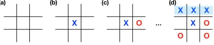
4.4. Tic-Tac-Toe. The Tic-Tac-Toe is a classical two-player board game, which is also
325
often played on pencil-and-paper. The “board” is a 3-by-3 grid with a total of 9 slots, as
illustrated in Fig. 5(a). At the beginning of the game, the board is empty. Then, the two
327
players take turn to mark any empty “slot” in each turn—typically one uses “X” the other
328
uses “O”. The player that is the first to have marked three consecutive horizontal, or vertical,
329
or diagonals slots, wins the game. For instance, Fig. 5(b-d) is an example of the sequence
330
of marks made by the players, where the first player (player “X”) eventually wins by having
331
marked an entire row (in this case, the top row). In general, if both players do their best at
332
every move, the outcome would be a draw.
Figure 5. Tic-Tac-Toe game. (a) Start of the game, where the board is made up of a 3-by-3 grid. (b-d) Example of a sequence of moves made by two players, where player “X” plays first, and eventually won the game by filling in an entire horizontal row.
333
Our interest here is not (re)analysis strategies of this relatively simple game. For those
334
who are interested, variants of the game actually has a connection to Ramsey theory, [11,22].
335
Here, we are intersted in testing our Boolean learning algorithm to see if it provides any useful
336
information. To this end, we collected the complete set of possible board configurations at
337
the end of a tic-tac-toe game, via the following link under the name “Tic-Tac-Toe Endgame
338
Data Set ”: https://archive.ics.uci.edu/ml/datasets/Tic-Tac-Toe+Endgame. There is a total
339
of 958 instances. For the t-th instance, we usex(t) = [x1(t), . . . , x9(t)]> to present the state 340
of the i-th slot, ordered as follows: upper-left, upper-middle, upper-right, middle-left, center,
341
middle-right, lower-left, lower-middle, and lower-right. Each xi(t) can either be 1 (if marked
342
by “X”), −1 (if marked by (“O”), or 0 (if empty). Corresponding to each instance t is the
343
final outcome, which we denote as y(t), which either equals 1 if player “X” wins or 0 if “X”
344
does not win. Interpreting(t) andy(t) as samples of random variablesX andY, we can ask
345
the question of which slots in the board, statistically, are more relevant (or predicative) for
346
the first player to win the game.
347
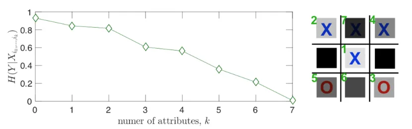
Applying our Boolean learning algorithm, we found a list of most important slots, ordered
348
in decreasing value of (added) relevance: i1 = 5 (the center),i2 = 1 (upper-left),i3= 9 (lower-349
right),i4 = 3 (upper-right),i5= 7 (lower-left),i6 = 8 (lower-middle), andi7 = 2 (lower-right). 350
To quantify the relative importance of each attribute, we compute the conditional entropy
351
H(Y|Xi1...ik) for k= 0, . . . ,7, whereH(Y|Xi0) is used to represent H(Y). This shows that, 352
as the number of attributes increases, uncertainty decreases monotonically and reaches 0
353
(complete predictability) when 7 attributes are used.
354
4.5. Risk Causality Analysis of Loans in Default Status. Loan default prediction is an
355
essential problem for the banks and insurance companies to fiscally responsibly approve loans.
356
However, in many cases, the borrowers fail to pay the loan as agreed, called loan default, which
357
motivates the risk analysis problem in the banking industry, to identify those parameters that
Figure 6. Decrease of uncertainty in “predicting” the outcome of a Tic-Tac-Toe game using partial ob-servations of the board in the final configuration. Here uncertainty is measured by the conditional entropy H(Y|Xi1...ik), and the indices ik are obtained using our Boolean inference algorithm: i1 = 5 (the center),
i2 = 1(upper-left), i3 = 9(lower-right), i4 = 3 (upper-right),i5 = 7(lower-left), i6 = 8(lower-middle), and i7= 2(lower-right).
identify one borrower as trustworthy, and another borrower as representing a high risk.
359
We consider the open dataset from LendingClub (American peer-to-peer lending
com-360
pany), which can be downloaded from LendingClub website. We considered the dataset for
361
the year 2019 (four quarters). The dataset contains more than 500,000 entries (data points,
362
sample size). However, we only considered the long term (the final) status of the loans.
There-363
fore, we excluded all the loans with the status “Current” as an outcome, to have a sample
364
size of 62,460 for our analysis. That is, all can be classified to and outcome “Paid in full”,
365
or “Default” status. We should emphasize here that we only considered the parameters as
366
Boolean in nature, which limits the considered to those 10 parameters that we investigate as
367
to their influence on the outcomes.
368
This example gives a causality driven description of those parameters thatcombined=, can
369
represent a high risk that the borrower will not be able to pay his loan in full. This causality
370
inference occurs within the Boolean framework for parameters concerning the loan long term
371
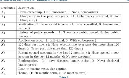
status. Table 3 shows the attributes and their description. In loan issuing risk analysis, the
372
amount of the requested loan and the annual income of the borrower are important variables
373
to consider, and they are both numeric variables. We introduce here the combined attribute,
374
loan to income ratio, which combines both variables in the form of a Boolean variable. Our
375
dataset has a sample size of 62,460, and the loan to income ratio range from 0.0001 to 36000.
376
So, we considered the median value µ ≈ 0.2 to be our threshold step, such that X9 = 0, 377
indicate that the loan to income ratio of the loan request is less than 0.2, and it is within the
378
lowest 50% of all the requested loans over the period (which is in our case, one year).
379
We then apply BoCSE, the proposed Boolean factors learning approach to the outcome
380
variableY, where we found that the relevant attributes are, in decreasing order of importance:
381 382
• X9, Loan to income ratio. 383
• X10, Loan terms. 384
We expect that the probability of having the loan fully paid (Y = 1) will be larger than a
386
default (Y = 0) in this example, for all the observed combinations of the relevant attributes.
387
However, the challenge here is to find the combination of attributes that, together represent
388
a high risk if approving the loan. For example, if for some attribute combinations (binary
389
string) X, the probability P r(Y = 1) = 0.8, and P r(Y = 0) = 0.2, we may not be satisfied
390
by saying that the expected outcome that the borrower will pay the loan in full because that
391
P r(Y = 1)> P r(Y = 0). Our focus here will be that there is a risk that the borrower will
392
not pay the loan with probability P r(Y = 0) = 0.2, which represents a high risk.
393
In Table4, we can see the inferred Boolean function relationship between these attributes
394
and the resulting outcomes. From application of our automated Boolean function learning
395
method, result shown in Table4 we summarize these interesting summary observations:
396
• The first four rows represent patterns whereX3= 0, that describe loans in which the 397
borrower’s income was not verified. We see that this feature coincides with a significant
398
increase in the probability that the loan will not be paid in full. The lowest value in this
399
group of patterns is (X3, X9, X10) = (0,0,1), which represents an unverified income, 400
low loan to income ratio, and 60 months loan term, and the joint probability is then
401
1.9%. We conclude that low loan to income ratio combined with long term loan (which
402
implies low monthly payment) reduces the risk of loan default.
403
• For the same pattern, but with a 36 months loan term, (X3, X9, X10) = (0,0,0), we see 404
a significant increase in risk from 1.9% to 9.6%. For the pattern (X3, X9) = (0,1),the 405
risk increases with the 36-month term loan, from 6.3% to 8.1%. This indicates that
406
higher monthly payments indicate a higher risk. However, the effect of the loan term
407
becomes neutral, meaning no effect in terms of observing only the verified income
408
patterns (X3 = 1). For these two patterns, where we have a verified income, the same 409
risk conclusions follow for both the 36 and 60 months terms loans.
410
• Comparing the above two points, we conclude that if the borrower’s reported income
411
is verified, there is no difference in the risk between different loan terms. However, if
412
it is not verified, then going with the 60 months term loans can profoundly reduce the
413
risk, regardless of the loan to income ratio.
414
• We see that the lowest risk, or the most trustworthy borrowers, are the ones with the
415
combination (X3, X9, X10) = (1,0,1), which represent a verified income, low loan to 416
income ratio, and 60 months term loan reflecting low monthly payments. The risk, in
417
this case, is about 0.4%. Unfortunately, however, such a pattern occurs infrequently,
418
representing fewer than 1% of the borrower customers.
419
• On the other hand, we see that a significant high risk associates with the combination
420
(X3, X9, X10) = (0,0,0), which represents unverified income, low LTI ratio, and 36 421
months term loan (high monthly payments). This is particularly interesting since a
422
low LTI may on its own may suggest a safer primary indication because it implies a
423
high income, low loan value, or both. However, we see that even with high income, or
424
low requested loan amount, the combination of unverified income together with large
425
monthly payment, (X3, X10) = (0,0), has the highest risk as compared to all other 426
combinations in the table, 9.6% and 8.1%.
attributes description
X1 Home ownership. (1: Homeowner, 0: Not a homeowner)
X2 Delinquency in the past two years. (1: Delinquency occurred, 0: No
Delinquency)
X3 Verification of the reported income. (1: Income verified, 0: Income not
verified)
X4 History of public records. (1: There is a public record, 0: No public
records.)
X5 Application type. (1: Individual, 0: With co-borrower)
X6 120 days past due. (1: Have account that ever past due more than 120
days, 0: Never past due more than 120 days.)
X7 Recent opened accounts in the last 12 months. (1: Have opened a new
account in the last 12 months, 0: No new accounts)
X8 Bankruptcies. (1: have declared bankruptcies, 0: Never declared
bankruptcies)
X9 Loan to income ratio. See caption.
X10 Terms. (1: 60 months term, 0: 36 months term)
Table 3
Attributes for the loan issuance data. All variables are Boolean. The outcomeY is a Boolean vector that take the value 1 if the loan fully paid, and 0 otherwise (charged off or marked as default). The loan to income
ratio is the ratior=the loan amount
annual income , and it is formed as a Boolean function such thatX9=
( 1, r > µ
0, r≤µ , where µis a threshold ratio that we selected to be the median value of the ratio of all the available dataset, and it was µ= 0.2.
5. Discussion and Conclusion. Although black-box machine learning methods become
428
increasingly more popular due to their relative ease to implement without deep understanding
429
of how they work, in some applications such as quantitative biology where it is essential
430
to uncover causal and relevant factors beyond functional fitting. A prototype problem of
431
such is to learn, from noisy observational data, the structure and function of a Boolean
432
network. The classic widely used REVEAL approach accomplishes this by performing a
433
combinatorial search in the space of Boolean variables, and its performance relies heavily
434
on having a relatively small network size and small maximum degree, two aspects that are in
435
sharp contrast to typical biological systems that can be large and complex. To overcome these
436
difficulties, here we present BoCSE as a new learning approach based on the optimization of
437
causation entropy applying to Boolean data. This new approach relies on computing entropies
438
of judiciously constructed subsets of variables, and does not require the combinatorial search
439
typically used in other methods. We benchmark effectiveness of BoCSE on random Boolean
440
networks, and further apply it in several real-world datasets, including in finding the minimal
441
relevant diagnosis signals, quantifying the informative signs of a board game Tic-Tac-Toe, and
442
in determining the causal signatures in loan defaults. In all examples, the BoCSE provides
443
outcomes that is directly interpretable and relevant to the respective application scenarios.
X3 X9 X10 Occurrence Po P r(Y = 0|X) P r(Y = 0, X)
0 0 0 38.75% 24.83% 9.6%
0 0 1 5.93% 33.66% 1.9%
0 1 0 23.29% 34.83% 8.1%
0 1 1 15.80% 39.92% 6.3%
1 0 0 4.35% 31.72% 1.4%
1 0 1 0.98% 38.59% 0.4%
1 1 0 5.78% 41.46% 2.4%
1 1 1 5.13% 46.28% 2.4%
Table 4
Inferred Boolean relations for the outcome variableY. Each entry in the “occurrence” column shows the fraction of observed attribute data(X3, X9, X10). Given each attribute pattern, the conditional probability that value of outcome P r(Y = 0|X = (x3, x9, x10)), meaning that the probability that the borrower will not fully pay the loan, is shown in theP r(Y = 0)column. The most important quantity that should be consider in the analysis is the joint probability for the pattern occurrence and the outcomeY = 0,P r(Y = 0, X= (x3, x9, x10)) is shown in last column of the table.
Appendix A. Basic concepts from information theory. In this appendix we review
445
some basic concepts from information theory. These concepts are rooted in information and
446
theory [24,6], and are heavily utilized in our computational approach for Boolean inference.
447
The (Shannon) entropyof a discrete random variable X is given by
448
(23) H(X) =−X
x
P(x) logP(x),
449
whereP(x) = Prob(X =x) and the summation is over the support of P(x), that is, all values
450
of x for which P(x) >0. The base of the “log” function is typically chosen to be 2 so that
451
the unit of entropy becomes “bit”, although other base values can also be used depending on
452
the application. Entropy is a measure of “uncertainty” associated with the random variable:
453
generally the larger the entropy is the more difficult it is to “guess” the outcome of a random
454
sample of the variable.
455
When two random variablesXandY are considered, we denote their joint distribution by
456
P(x, y) = Prob(X=x, Y =y) and conditional distributions byP(y|x) = Prob(Y =y|X=x)
457
and P(x|y) = Prob(X =x|Y =y), respectively. These functions are used to define thejoint 458
entropyas well as the conditional entropies, as:
459
(24)
Joint entropy: H(X, Y) =−P
x,yP(x, y) logP(x, y), Conditional entropies:
Y given X:H(Y|X) =−P
x,yP(x, y) logP(y|x), X given Y:H(X|Y) =−P
x,yP(x, y) logP(x|y).
460
While the joint entropy H(X, Y) measures the uncertainty associated with the joint variable
461
(X, Y), the conditional entropy H(Y|X) measures the uncertainty of Y given knowledge
462
about X and similar interpretation holds for H(X|Y). In general, H(Y|X) ≤ H(Y) and
H(X|Y) ≤ H(X), with “=” if and only if X and Y are independent. Interestingly, the
464
reduction of uncertainty as measured by H(Y)−H(Y|X) coincides with H(X)−H(X|Y),
465
leading to a quantity called the themutual information (MI) betweenX and Y, given by:
466
(25) I(X;Y) =H(X)−H(X|Y) =H(Y)−H(Y|X).
467
Mutual information is symmetricI(X;Y) =I(Y;X), and also nonnegative: I(X;Y)≥0 with
468
I(X;Y) = 0 if and only if X and Y are independent.
469
Finally, theconditional mutual information (CMI) betweenX and Y given Z is
470
(26) I(X;Y|Z) =H(X|Z)−H(X|Y, Z),
471
which measures the reduction of uncertainty ofX given Z due to extra information provided
472
by Y. Conditional mutual information is symmetric with respect to interchangingX and Y,
473
and nonnegative, equalling zero if and only if the conditional probabilitiesP(x|z) andP(y|z)
474
are independent: P(x|z)P(y|z) =P(x, y|z).
475
REFERENCES 476
[1] M. C. ´Alvarez-Silva, S. Yepes, M. M. Torres, and A. F. G. Barrios,Proteins interaction network
477
and modeling of igvh mutational status in chronic lymphocytic leukemia, Theoretical Biology and
478
Medical Modelling, 12 (2015), p. 12.
479
[2] E. Azpeitia, J. Davila-Velderrain, C. Villarreal, and E. R. Alvarez-Buylla,Gene regulatory
480
network models for floral organ determination, in Flower Development, Springer, 2014, pp. 441–469.
481
[3] N. Berestovsky and L. Nakhleh,An evaluation of methods for inferring boolean networks from
time-482
series data, PLoS One, 8 (2013), p. e66031.
483
[4] C. Campbell, S. Yang, R. Albert, and K. Shea, A network model for plant–pollinator community
484
assembly, Proceedings of the National Academy of Sciences, 108 (2011), pp. 197–202.
485
[5] K. J. Cios and L. A. Kurgan,Hybrid inductive machine learning: An overview of clip algorithms, in
486
New Learning Paradigms in Soft Computing, Springer, 2002, pp. 276–322.
487
[6] T. M. Cover and J. A. Thomas,Elements of information theory, John Wiley & Sons, Hoboken, New
488
Jersey, 2 ed., 2006.
489
[7] J. Czerniak and H. Zarzycki,Application of rough sets in the presumptive diagnosis of urinary system
490
diseases, in Artificial intelligence and security in computing systems, Springer, 2003, pp. 41–51.
491
[8] M. I. Davidich and S. Bornholdt,Boolean network model predicts cell cycle sequence of fission yeast,
492
PloS one, 3 (2008), p. e1672.
493
[9] C. Ding and H. Peng, Minimum redundancy feature selection from microarray gene expression data,
494
Journal of bioinformatics and computational biology, 3 (2005), pp. 185–205.
495
[10] ˚A. Flobak, A. Baudot, E. Remy, L. Thommesen, D. Thieffry, M. Kuiper, and A. Lægreid,
496
Discovery of drug synergies in gastric cancer cells predicted by logical modeling, PLoS computational
497
biology, 11 (2015), p. e1004426.
498
[11] S. W. Golomb and A. W. Hales,Hypercube tic-tac-toe, More Games of No Chance, 42 (2002), pp. 167–
499
180.
500
[12] S. R. Hegde, H. Rajasingh, C. Das, S. S. Mande, and S. C. Mande,Understanding communication
501
signals during mycobacterial latency through predicted genome-wide protein interactions and boolean
502
modeling, PLoS One, 7 (2012), p. e33893.
503
[13] T. Helikar, N. Kochi, J. Konvalina, and J. A. Rogers,Boolean modeling of biochemical networks,
504
The Open Bioinformatics Journal, 5 (2011), pp. 16–25.
505
[14] I. Irurzun-Arana, J. M. Pastor, I. F. Troc´oniz, and J. D. G´omez-Mantilla, Advanced boolean
506
modeling of biological networks applied to systems pharmacology, Bioinformatics, 33 (2017), pp. 1040–
507
1048.
[15] L. A. Kurgan, K. J. Cios, R. Tadeusiewicz, M. Ogiela, and L. S. Goodenday,Knowledge discovery
509
approach to automated cardiac spect diagnosis, Artificial intelligence in medicine, 23 (2001), pp. 149–
510
169.
511
[16] H. L¨ahdesm¨aki, I. Shmulevich, and O. Yli-Harja,On learning gene regulatory networks under the
512
boolean network model, Machine learning, 52 (2003), pp. 147–167.
513
[17] F. Li, T. Long, Y. Lu, Q. Ouyang, and C. Tang,The yeast cell-cycle network is robustly designed,
Pro-514
ceedings of the National Academy of Sciences of the United States of America, 101 (2004), pp. 4781–
515
4786.
516
[18] S. Liang, S. Fuhrman, and R. Somogyi,Reveal, a general reverse engineering algorithm for inference
517
of genetic network architectures, in Pacific Symposium on Biocomputing, vol. 3, 1998, pp. 18–29.
518
[19] H. Liu, F. Zhang, S. K. Mishra, S. Zhou, and J. Zheng,Knowledge-guided fuzzy logic modeling to
519
infer cellular signaling networks from proteomic data, Scientific reports, 6 (2016), p. 35652.
520
[20] D. MacLean and D. J. Studholme,A boolean model of the pseudomonas syringae hrp regulon predicts
521
a tightly regulated system, PloS one, 5 (2010), p. e9101.
522
[21] S. Marshall, L. Yu, Y. Xiao, and E. R. Dougherty,Inference of a probabilistic boolean network
523
from a single observed temporal sequence, EURASIP Journal on Bioinformatics and Systems Biology,
524
2007 (2007), pp. 5–5.
525
[22] O. Patashnik,Qubic: 4×4×4 tic-tac-toe, Mathematics Magazine, 53 (1980), pp. 202–216.
526
[23] K. Raman, A. G. Bhat, and N. Chandra,A systems perspective of host–pathogen interactions:
pre-527
dicting disease outcome in tuberculosis, Molecular BioSystems, 6 (2010), pp. 516–530.
528
[24] C. E. Shannon,A mathematical theory of communication, Bell System Tech. J., 27 (1948), pp. 379–423,
529
623–656.
530
[25] S. N. Steinway, M. B. Biggs, T. P. Loughran Jr, J. A. Papin, and R. Albert,Inference of network
531
dynamics and metabolic interactions in the gut microbiome, PLoS computational biology, 11 (2015),
532
p. e1004338.
533
[26] J. Sun and E. M. Bollt,Causation entropy identifies indirect influences, dominance of neighbors and
534
anticipatory couplings, Physica D: Nonlinear Phenomena, 267 (2014), pp. 49–57.
535
[27] J. Sun, C. Cafaro, and E. M. Bollt,Identifying the coupling structure in complex systems through
536
the optimal causation entropy principle, Entropy, 16 (2014), pp. 3416–3433.
537
[28] J. Sun, D. Taylor, and E. M. Bollt,Causal network inference by optimal causation entropy, SIAM
538
Journal on Applied Dynamical Systems, 14 (2015), pp. 73–106.
539
[29] J. Thakar and R. Albert, Boolean models of within-host immune interactions, Current opinion in
540
microbiology, 13 (2010), pp. 377–381.
541
[30] A. Veliz-Cuba, An algebraic approach to reverse engineering finite dynamical systems arising from
542
biology, SIAM Journal on Applied Dynamical Systems, 11 (2012), pp. 31–48.
543
[31] F. Vitali, L. D. Cohen, A. Demartini, A. Amato, V. Eterno, A. Zambelli, and R. Bellazzi,
544
A network-based data integration approach to support drug repurposing and multi-target therapies in
545
triple negative breast cancer, PloS one, 11 (2016), p. e0162407.
546
[32] S. Von der Heyde, C. Bender, F. Henjes, J. Sonntag, U. Korf, and T. Beissbarth, Boolean
547
erbb network reconstructions and perturbation simulations reveal individual drug response in different
548
breast cancer cell lines, BMC systems biology, 8 (2014), p. 75.