Automated Glaucoma Detection Techniques Using
Fundus Image
Rohan Appasaheb Borgalli, Hari Pratap Gautam,Winner George Parayil
(Assistant Professor) Electronics and Telecommunications Dept., Shah and Anchor Kutchhi Engineering College, Mumbai, India; (Assistant Professor) Electronics and Telecommunications Dept., K.N.G.D Modi Engineering College, Delhi, India;
(Assistant Professor) Electronics and Telecommunications Dept., St. John College of Engineering and Technology, Thane, In-dia.
Email: [email protected], [email protected], [email protected].
ABSTRACT: This paper presents automated glaucoma detection techniques based on neural network and Adaptive Neuro fuzzy Inference system (AN-FIS) Classifier. Digital image processing techniques, such as preprocessing, morphological operations and thresholding, are widely used for the auto-matic detection of optic disc, blood vessels and computation of the features of fundus image. Glaucoma is a disease of the optic nerve caused by the increase in the intraocular pressure of the eye. Glaucoma mainly affects the optic disc by increasing the cup size. It can lead to the blindness if it is not detected and treated in proper time. The detection of glaucoma through Optical Coherence Tomography (OCT) and Heidelberg Retinal Tomography (HRT) is very expensive, this limitation is removed by this Glaucoma Diagnosis system with good performance. In addition to diagnosis of Glaucoma a Graphical user interface (GUI) is developed. This GUI is used for automatic diagnosing and displaying the diagnosis result in a more friendly user inter-face The results presented in this paper indicate that the features are clinically significant in the detection of glaucoma. Proposed system of this paper is able to classify the glaucoma automatically with a sensitivity and specificity of 98% and 95% respectively.
Keywords : Intra ocular pressure, Ocular Computing Tomography, Heidelberg Retinal Tomography, Cup to Disk Ratio, Support Vector System, Artificial Neural Network.
1 INTRODUCTION
This paper presents automated glaucoma detection techniques. Glaucoma is the second leading cause of blindness with an estimated 60 million glaucomatous cases globally in 2012 [1], and it is responsible for 5.2 million cases of blindness [2]. In India, the prevalence of glaucoma is 3-4% in adults aged 40 years and above, with more than 90% of the patients unaware of the condition [3] [4]. Clinically, glaucoma is a chronic eye condition in which the optic nerve is progressively damaged. Patients with early stages of glaucoma do not have symptoms of vision loss. As the disease progresses, patients will encounter loss of peripheral vision and a resultant “tunnel vision”. Late stage of glaucoma is associated with total blindness. As the optic nerve damage is irreversible, glaucoma cannot be cured. However, treatment can prevent progression of the disease. Therefore, early detection of glaucoma is crucial to prevent blindness from the disease. The digital color fundus image is a more cost effective imaging modality to assess optic nerve damage compared to HRT and OCT, and it has been widely used in recent years to diagnose various ocular diseases, including glaucoma. In this work, we will present a system to diagnose glaucoma from fundus images with MATLAB based Graphic User Interface (GUI) tool is developed for analysis of fundus image by the ophthalmologist for detection of Glaucoma.
2
S
TRUCTUREO
FE
YEA
NDE
YER
ELATEDD
ISEASESThis section start with discussion on the anatomy of the eye and the functioning of the eye followed by eye related diseas-es Glaucoma is ddiseas-escribed in detail.
2.1 Anatomy of Eye
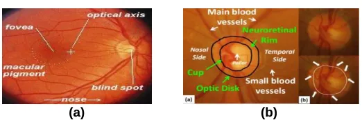
The anatomy of the human eye is presented in Fig 1.This illustrates a cross sectional view of the human eye with various ocular structures indicated. Basically, the human eye functions in a sequential manner. Firstly, the lights perceived will pass through the cornea and pupil to the lens (which is surrounded by the iris). Secondly, the lens will focus the lights
onto the retina. Thirdly, the captured light is converted into signals. Finally the signals are transmitted to the brain, through the optic nerve, where the signals are perceived as images. With respect to the work described in this paper only a small number of the anatomical parts illustrated in Fig 1 are important, these are highlighted in the figure using red coloured labels. The retina is a thin layer located on the inside wall at the back of human eye, between the choroid and the vitreous body (the vitreous body is a clear gel posterior to the lens). The retina is composed of photoreceptors (rods and cones) and neural tissues that receives light, converts it into neural
Figure 1Anatomy of Eye
communicate perceived signals to the brain through the optic nerve. Its horizontal and vertical diameters" are approximate-ly1.7 mm and 1.9 mm respectively . The optic disc contains no photoreceptorand thus represents a psychological blind spot". The optic disc is clearly visiblewithin retinal images as shown in Figure 1.3 where the optic disc is the bright yellowcircle from which veins and arteries can be seen to emanate. The optic disc's locationwithin an image, together with the blood vessels, can be used to indicate whether theimage is of a left or right eye (the optic disc is located next to the subject's nose). Notethat the blood vessels are responsible for providing the nutrients required by the inner parts of the retina.
2.2 Background of Glaucoma
Glaucoma is a disease of progressive optic neuropathy with loss of retinal neurons and the nerve fibre layer, resulting in blindness if left untreated. Glaucoma describes a group of dis-eases that kill retinal ganglion cells. “High IOP is the strongest known risk factor for glaucoma but it is neither necessary nor sufficient to induce the neuropathy.” Glaucoma is a group of diseases that can damage the eye's optic nerve and result in vision loss and blindness. There is a dose-response relation-ship between intraocular pressure and the risk of damage to the visual field. Glaucoma is a disease that damages the eye‟s optic nerve. The optic nerve is connected to the retina (a layer of light-sensitive tissue lining the back of the eye) and is made up of many nerve fibres, like an electric cable is made up of many wires. It is the optic nerve that sends signals from eye retina to the brain, where these signals are interpreted as the images you see.
Images of Eye Used in Glaucoma Assessment
There are two type of image of eye used for Glaucoma As-sessment
A. Fundus image B. Retinal image
(a) (b)
Figure 2 (a) Fundus Image of eye (b) Retinal Image of eye
3 CONVENTIONAL TECHNIQUE USED FOR GLAUCOMA
There are various type of technique for glaucoma assessment according to parameter changed some technique are as fol-lows.
3.1 Optical coherence tomography (OCT)
Optical Coherence Tomography (OCT) is an optical imaging modality that uses near-infrared light to create high-resolution images of tissue microstructure. OCT is a sensitive non-invasive tool in detecting and quantifying the macular thick-ness. OCT is a new, noninvasive on contact, transpupillary imaging technology which can image retinal structures in vivo with a resolution of 10 to 17 microns. Cross-sectional images of the retina are produced using the optical backscattering of light in a fashion analogous to B- scan ultra-sonography. The
anatomic layers within the retina can be differentiated and reti-nal thickness can be measured [9].
3.2 Heidelberg retina tomography (HRT)
The Heidelberg Retina Tomography (HRT) is a confocal scan-ning laser ophthalmoscope that is capable of acquiring and analyzing three dimensional images of the optic nerve head and per papillary retina. It provides topographic measurements of the optic nerve head including the size, shape and contour of the optic disc, neuro-retinal rim, optic cup and measure-ments of the per papillary retina and nerve fibre layer. The typ-ical application of the HRT is the assessment of the glaucoma-tous optic nerve head. The HRT also uses an imaging tech-nique called „scanning laser „tomography‟, in which a laser light scans the retina sequentially, starting from above the reti-nal surface then through the retina at increasing depths [10].
3.3 Color fundus imaging (CFI)
The device produces a color fundus image of the retina. The image produced is an ultra wide field, high contrast optomap image that can aid in detecting and documenting retinal health. The optomap image allows viewing of up to 200 inter-nal degrees of the fundus in one image. Along with a screen-ing tool for early detection of diseases or abnormalities it can be used to facilitate the diagnosis and management of ocular pathology [11].
3.4 Medical Image Processing for Glaucoma detection In this section some of the principles applied in this research work are included. These principles include: Color Space Con-version, Histogram Equalization, K-mean Clustering Algorithm, Classification, Image Morphological Operations and Skeleton-ization [12].
4 PROPOSED METHOD FOR CLASSIFICATION
In this section proposed classification technique is described which is based on Neural Network and Adaptive Fuzzy Infer-ence system (ANFIS). So first of all neural network will explain in detail.
4.1 Delta Rule
The delta rule is a gradient descent learning rule for updating the weights of the artificial neurons in a single-layer percep-tron. It is a special case of the more general back propagation algorithm. For a neuron j with activation function g(x) the delta rule for j's ith weight Wij is given by Equation 4.1
j
j j ij
j j
i j
x
E
E
EA
EI W
y
x
i
(4.1) Where,
α small constant called learning rate g(x) is the neuron's activation function tj is the target Output
hj is the weighted sum of the neuron's inputs yj is the actual output xj is the ith input
j i ji
h
x w
(4.2))
(
jj
g
h
y
(4.3)The delta rule is commonly stated in simplified form for a per-ceptron with a linear activation function in equation 4.4
( ,j j) i
ji t y x
w
(4.4) The delta rule is derived by attempting to minimize the error in the output of the perceptron through gradient descent. The error for a perceptron with j outputs can be measured (Equa-tion 4.5).
2 1
2
1
=
E
t
jy
j (4.5)In this case, we wish to move through weight space of the neuron (the space of all possible values of all of the neuron's weights) in proportion to the gradient of the error function with respect to each weight. In order to do that, we calculate the partial derivative of the error with respect to each weight. Be-cause, we are only concerning ourselves with the jth neuron, we can substitute the error formula above while omitting the summation (Equation 4.6):
2j j
i
ji ji ji
1
t y
E 2 y
w w w
(4.6)
4.2 Back propagation algorithm
Back propagation is a form of supervised learning for multi-layer nets, also known as the generalized delta rule. Error data at the output layer is back propagated to earlier ones, allowing incoming weights to these layers to be updated. It is most of-ten used as training algorithm in current neural network appli-cations. The back propagation algorithm has been widely used as a learning algorithm in feed forward multilayer neural net-works.
a. Learning with the back propagation algorithm
The back propagation algorithm is an involved mathematical tool; however, execution of the training equations is based on iterative processes, and thus is easily implement able on a computer. [8]
Weight changes for hidden to output weights just like Widrow-Hoff learning rule.
Weight changes for input to hidden weights just like Widrow-Hoff learning rule bu error signal is obtained by "back-propagating" error from the output units
During the training session of the network, a pair of patterns is presented (Xk, Tk), where Xk in the input pattern and Tk is the target or desired pattern. The Xk pattern causes output re-sponses at teach neurons in each layer and, hence, an output Ok at the output layer. At the output layer, the difference be-tween the actual and target outputs yields an error signal. This error signal depends on the values of the weights of the
neu-rons I each layer. This error is minimized, and during this pro-cess new values for the weights are obtained. The speed and accuracy of the learning process-that is, the process of updat-ing the weights-also depends on a factor, known as the learn-ing rate.Before startlearn-ing the back propagation learnlearn-ing process, we need the following:
The set of training patterns, input, and target
A value for the learning rate
A criterion that terminates the algorithm
A methodology for updating weights
The nonlinearity function (usually the sigmoid)
Initial weight values (typically small random values)
b. Implementation of back propagation algorithm
The back-propagation algorithm consists of the following steps:
Each Input is then multiplied by a weight that would either inhibit the input or excite the input. The weighted sum of then inputs in then calculated
First, it computes the total weighted input Xj, using the formu-la:
j i ij
i
X
y W
(4.7)
Where,
Yi is the activity level of the j th
unit in the previous layer and Wij
is the weight of the connection between the ith and the jth unit. Then the weighed Xj is passed through a sigmoid function that
would scale the output in between 0 and 1.
Next, the unit calculates the activity yj using some
function of the total weighted input. Typically we use the sigmoid function:
( )
1 / (1
xj)
j
y
e
(4.8) Once the output is calculated, it is compared with the required output and the total Error E is computed
Once the activities of all output units have been de-termined, the network compute the error E, which is defined by the expression:
2
)
(
2
1
=
E
jy
j
d
j (4.9)Where yj is the activity level of the ith unit in the top layer and dj is the desired output of the ith unit.) Now the error is propagated backwards.
1. Compute how fast the error changes as the activity of an output unit is changed. This error derivative (EA) is the differ-ence between the actual and the desired activity.
j j j
j E
EA y d
y
(4.10)
of a unit changes as its total input is changed.
(1
)
j
j j j j
j j j
y
E
E
EI
EA y
y
x
y
x
(4.11)3. Compute how fast the error changes as a weight on the connection into an output unit is changed. This quantity (EW) is the answer from step 2 multiplied by the activity level of the unit from which the connection emanates.
j
j j j i
ij j ij
x
E
E
EW
EI
EI y
W
x
W
(4.12)4. Compute how fast the error changes as the activity of a unit in the previous layer is changed. This crucial step allows back propagation to be applied to multi-layer networks. When the activity of a unit in the previous layer changes, it affects the activities of all the output units to which it is connected. So to compute the overall effect on the error, we add together all these separate effects on output units. But each effect is sim-ple to calculate. It is the answer in step 2 multiplied by the weight on the connection to that output unit
j
j j ij
j j
i j
x
E
E
EA
EI W
y
x
i
(4.13)By using steps 2 and 4, we can convert the EA‟s of one layer of units into EA‟s for the previous layer. This procedure can be repeated to get the EA‟s for as many previous layers as de-sired. Once we know the EA of a unit, we can use steps 2 and 3 to compute the EW‟s on its incoming connections.
4.3 Adaptive Neuro-Fuzzy Inference System as Clas-sifier (ANFIS)
Adaptive Neuro-Fuzzy Inference Systems combines the learn-ing capabilities of neural networks with the approximate rea-soning of fuzzy inference algorithms. ANFIS uses a hybrid learning algorithm to identify the membership function parame-ters of Sugeno type fuzzy inference systems. The aim is to develop ANFIS-based learning models to classify normal and abnormal images from fundus image to detect glaucoma .An adaptive neural network is a network structure consisting of five layers and a number of nodes connected through direc-tional links. The first layer executes a fuzzification process, second layer executes the fuzzy AND of the antecedent part of the fuzzy rules, the third layer normalizes the fuzzy member-ship functions, the fourth layer executes the consequent part of the fuzzy rules and finally the last layer computes the output of the fuzzy system by summing up the outputs of the fourth layer [24].Each node is characterized by a node function with a fixed or adjustable parameter. Learning or training phase of a neural network is a process to determine parameter values to sufficiently fit the training data. Based on this observation a hybrid learning rule is employed in this thesis which combines the gradient descent and the least-square method to find a feasible set of antecedent and consequent parameters. Adap-tive Neuro Fuzzy Inference System (ANFIS) is the combination
of ANN and the fuzzy logic ANFIS is a multilayer feed forward network which uses ANN learning algorithms and fuzzy rea-soning to characterize an input space to an output .Takagi and Sugeno proposed the first systematically fuzzy modeling. The ANFIS approach uses Gaussian functions for fuzzy sets and linear functions for the rule outputs The parameters of the network are the mean and standard deviation of the member-ship functions (antecedent parameters) and the coefficients of the output linear functions.
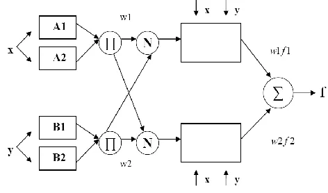
a. ANFIS Architecture
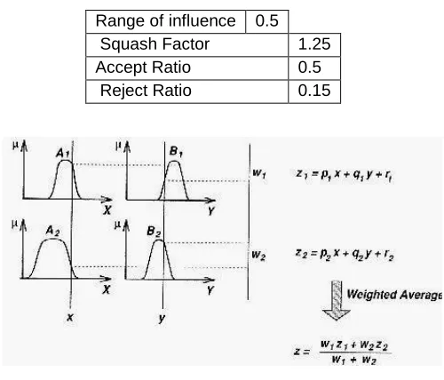
In ANFIS, Takagi-Sugeno type fuzzy inference system is used. The output of each rule can be a linear combination of input variables plus a constant term or can be only a constant term. The final output is the weighted average of each rule‟s output. Basic ANFIS architecture that has two inputs x and y and one output z is shown in Figure 3.2 The rule base contains two Takagi-Sugeno if then rules as follows
Rule 1. If x is A1 and y is B1, then
f
1
p x
1
q y
1
r
1Figure 3ANFIS Architecture
Rule 2. If x is A2 and y is B2 , then
f
2
p x
2
q y
2
r
2b. ANFIS learning algorithm
From the proposed ANFIS architecture above (Figure 4.6.6), the output f can be defined as
1 2 1 2 1 2 1 2
w
w
f
f
f
w
w
w
w
Figure 4 Takagi-Sugeno Fuzzy Inference System
)
(
)
(
1 1 1 2 2 2 21
p
x
q
y
r
w
p
x
q
y
r
w
f
(4.14)2 2 2 2 2 2 1 1 1 1 1
1
)
(
)
(
)
(
)
(
)
(
)
(
w
x
p
w
y
q
w
r
w
x
p
w
y
q
w
r
f
Where p1, q1, r1, p2 , q2 and r2 are the linear consequent parameters. The methods for updating the parameters are listed as below:
2. Gradient decent and One pass of Least Square Estimates (LSE): The LSE is applied only once at the very beginning to get the initial values of the consequent parameters and then the gradient descent takes over to update all pa-rameters.
3. Gradient and LSE: This is the hybrid learning rule.
Since the hybrid learning approach converges much faster by reducing search space dimensions than the original back propagation method, it is more desirable. In the forward pass of the hybrid learning, node outputs go forward until layer 4 and the consequent parameters are identified with the least square method. In the backward pass, the error rates propa-gate backward and the premise parameters are updated by gradient descent Parameters used for clustering are shown in Table-I
TABLE-I Parameter used for clustering
Range of influence 0.5 Squash Factor 1.25 Accept Ratio 0.5 Reject Ratio 0.15
5 RESULT AND SIMULATION
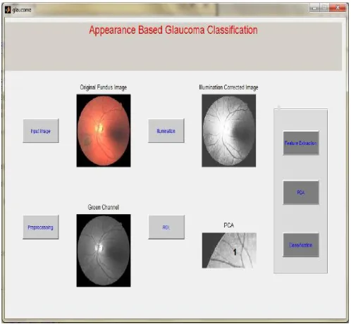
In this chapter experimental results are presented in support of the claims made about the proposed methods in the earlier chapters. The simulations were performed using MATLAB R2010a.For the simulation the images are used from Origa image database
5.1 Image pre-processing Result
In the processing of input image various type of pre-processing is applied which is described in earlier chap-ter.Results of pre-processed image are as follows.
Image illumination correction results
(a) (b)
(c) (d)
Fig 5 (a) original image (b)Green channel of original image (c) illumination corrected image (d) ROI cropped Image
Feature extraction result and performance analysis In this section extracted feature are calculated which is result of used method. First result of cup detection analysis
Optic cup detection
1. To assess the area overlap between the computed region and ground truth of the optic cup pixel wise precision and re-call values are computed
FP
TP
TP
ecision
Pr
(5.1)FN
TP
TP
call
Re
(5.2)Where TP is the number of True positives, FP is the number of false positive and FN is the number of false negative pixels.
2. Another method of evaluating the performance is using F
Score given by
)
Re
(Pr
Re
*
Pr
*
2
call
ecision
call
ecision
F
(5.3)Value of F score lies between 0 – 1 and score will be high for an accurate method. Average F score for thresholding and component analysis are compared and listed in Table II.
TABLE II: F score for cup segmentation
Images Threshold Component
analysis Proposed
1 .67 .72 .82
2 .69 .76 .89
3 .66 .74 .86
4 .63 .70 .81
5 .54 .69 .79
Figure6GUI of Proposed Glaucoma diagnosis system
TABLE III: Performance Analysis of Features
Features Sensitivity (%) Specificity (%) Accuracy (%) Cup to disk
ratio 93.5 95.3 94.2
Pixel intensity
value 96.1 94.3 97.2
fft coefficient 92.5 93.6 95.5
B-spline
coef-ficient 93.8 96.5 99.2
5.2 Classification Results and analysis
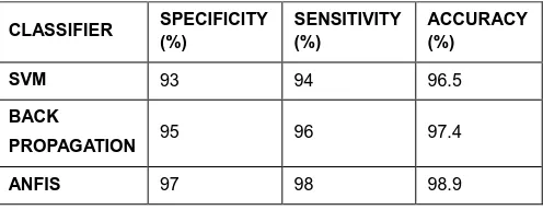
Classifiers namely ANFIS, SVM and Back Propagation Neural network are used to classify between normal and abnormal cases of glaucoma. Parameters that are used for generating Fuzzy Inference System (FIS) are shown in Table-IV. ANFIS integrates the learning capabilities of neural networks with approximate reasoning of fuzzy inference algorithms [11].
Performance Measure of Classifiers
The system is trained and tested for a dataset shown in Table-III. Classification accuracy is the ratio of the total number of correctly classified images to total number of misclassified images [11]. Table IV shows the Classification Accuracy of the classifiers that shows that the proposed method has the high-est classification rate with SVM as classifier. The classification accuracy achieved by ANFIS, SVM and Back Propagation is also shown in this table.In this work 50 images are used for training and 100 images for testing. 150 images, 50 from each of the class for training and 100 images (50 normal, and 50 abnormal) for testing were used for classification.
TABLE IV: Dataset for Fundus Image Classification
Category No. of train-ing Images
No. of testing Images
No. of Imag-es/Class
Normal 50 100 150
Abnormal 50 100 150
Total 100 200 300
Classification accuracy
Classification accuracy is the ratio of the total number of cor-rectly classified images to the, total number of misclassified images. Table-V shows the performance measure of the clas-sifiers and classifier accuracy.A screened fundus is considered as a true positive (TP) if the fundus is really abnormal and if the screening procedure also classified it as abnormal. Simi-larly, a true negative (TN) means that the fundus is really nor-mal and the procedure also classified it as nornor-mal. A false pos-itive (FP) means that the fundus is really normal, but the pro-cedure classified it as abnormal. A false negative (FN) means that the procedure classified the screened fundus as normal, but it really is abnormal. Sensitivity is the percentage of ab-normal funduses classified as abab-normal by the procedure.
TABLE V: Classification Accuracy of Classifiers
CCI MI CA CCI MI CA CCI MI CA
Normal 100 93 7 93 95 5 95 97 3 97
Abnormal 100 94 6 94 96 4 96 98 2 98
Category
No. of
Test Images
SVM Back
Propogation ANFIS
CCI = Correctly Classified Images, MI = Misclassified Images, CA = Classification Accuracy (in %)
Sensitivity =
TP
TP
FN
(5.4)Specificity is the percentage of normal funduses classified as normal by the procedure.
Specificity =
TN
TABLE VI: Performance Measure of the Classifier
TABLE VII: Classification Rate of Classifiers
The higher the sensitivity and specificity values, the better the procedure. Performance of each classifier is measured in terms of sensitivity, specificity, and accuracy. Sensitivity is a measure that determines the probability of results that are true positive such that the person has glaucoma. Specificity is a measure that determines the true negatives that the person is not affected by glaucoma. Accuracy is a measure that deter-mines the results that are accurately classified. The same da-taset is used for neural network based Back propagation clas-sifier. MATLAB (version 2010 a) is used for implementation of the work. Comparative analysis performed between the classi-fiers based on correctly classified images, is shown in Table-VI and Table-VII From above result analysis it can be shown that the performance of ANN and ANFIS classifier improved with respect to SVM classifier in terms of sensitivity, specificity and accuracy and we can conclude that proposed classifiers gives better Performance in comparison of SVM classifier. Classifi-cation rate is also improved by the proposed classifier.
6
CONCLUSION
In this paper an appearance based Glaucoma diagnosis sys-tem is developed for detection of glaucoma abnormal eyes through fundus images using image processing techniques and neural network algorithm. k means clustering provides a promising step for the accurate detection of optic cup bounda-ry.Proposed classification technique which is based on ANFIS and neural network achieves good classification accuracy with a smaller convergence time compared to support vector ma-chine classifier. Performance of the proposed approach is comparable to human medical experts in detecting glaucoma. Proposed system combines feature extraction techniques with segmentation techniques for the diagnosis of the image as normal and abnormal. The method of the considering features like B-spline coefficient, FFT coefficient, cup to disk ratio can be used as an additional feature for distinguishing between normal and glaucoma or glaucoma suspects. The proposed system can be integrated with the existing ophthalmologic tests and clinical assessments in addition to other risk factors according to a determined clinical procedure and can be used in local health camps for effective screening.
REFERENCES
[1] H.A. Quigley and A.T. Broman, "The number of people with glaucoma worldwide in 2010 and 2020," Br J Ophthalmology, vol. 90, pp. 262-7, Mar 2006.
[2] B. Thylefors and A.D. Negrel, "The global impact of glaucoma," Bull World Health Organ, vol. 72, no. 3, pp. 323-6, 1994.
[3] S.Y. Shen et al., "The prevalence and types of glaucoma in Ma-lay people: the Singapore MaMa-lay eye study," Invest Ophthalmol-ogy Vis Sci,vol. 49, no. 9, pp. 3846-51, 2008.
[4] P.J. Foster et al., "The prevalence of glaucoma in Chinese resi-dents of Singapore: a cross-sectional population survey of the Tanjong Pagar district," Arch Ophthalmol, vol. 118, no. 8, pp. 1105-11, 2000.
[5] D.H. Sim and L.G. Goh, "Screening for glaucoma in the Chinese elderly population in Singapore," Singapore Med J, vol. 40, no. 10, pp. 644-7, 1999.
[6] Congdon, N., et al. “Eye Diseases Prevalence Research Group. „Causes and Prevalence of Visual Impairment among Adults in the United States.” Archives of Ophthalmology 122.4 (2004): 477-85.
[7] Betz, P., Camps, F., Collignon-Brach, J., Lavergne, G., Weekers, R., 1982. Biometric study of the disc cup in open-angle glauco-ma. Graefes Arch. Clin. Exp. Ophthalmol. 218 (2), 70–74.
[8] Quillen, D. A. “Common Causes of Vision Loss in Elderly Pa-tients.” American Family Physician 60.1 (1999): 99-108.
[9] Medeiros, F.A., Zangwill, L.M., Bowd, C., Weinreb, R.N., 2004b. Comparison of the GDx VCC scanning laser polarimeter, HRT II confocal scanning laser ophthalmoscope, and stratus OCT opti-cal coherence tomograph for the detection of glaucoma. Arch. Ophthalmol. 122 (6), 827–837.
[10]Staal, J., Abràmoff, M., Niemeijer, M., Viergever, M., van Ginneken, B., 2004. Ridge based vessel segmentation in color images of the retina. IEEE Trans. Med. Imag. 23 (4), 501–509.
[11]Burgansky-Eliash, Z., Wollstein, G., Bilonick, R.A., Ishikawa, H., Kagemann, L., Schuman, J.S., 2007. Glaucoma detection with the Heidelberg Retina Tomograph (HRT) 3. Ophthalmology 114 (3), 466–471.
[12]Rafael C. Gonzalez and Richard E. Woods. ‘Digital Image Pro-cessing using MATLAB’ 2nd edition. Prentice Hall, 2002. ISBN 0-201-18075-8.
[13]Narasimha-Iyer, H., Can, A., Roysam, B., Stewart, C.V., Tanen-baum, H.L., Majerovics, A., Singh, H., 2006. Robust detection and classification of longitudinal changes in color retinal fundus images for monitoring diabetic retinopathy. IEEE Trans. Biomed. Eng. 53 (6), 1084–1098.
[14]Meier, J., Bock, R., Michelson, G., Nyúl, L.G., Hornegger, J., 2007. Effects of preprocessing eye fundus images on appear-CLASSIFIER SPECIFICITY
(%)
SENSITIVITY (%)
ACCURACY (%)
SVM 93 94 96.5
BACK
PROPAGATION 95 96 97.4
ANFIS 97 98 98.9
Classifier Normal (%) Abnormal (%)
SVM 94.3 93.5
ANN 95.6 94.5
ance based glaucoma classification. In: 12th International Con-ference on Computer Analysis of Images and Patterns, CAIP. Lecture Notes in Computer Science (LNCS), vol. 4673/2007, Berlin, pp. 165–173.
[15]Canny, J.F., 1986. A computational approach to edge detection. IEEE Trans. Pattern Anal. Mach. Intell. 8 (6), 679–698.
[16]Bertalmio, M., Sapiro, G., Caselles, V., Ballester, C., 2000. Im-age inpainting. In: Proceedings of the 27th Annual Conference on Computer Graphics and Interactive Techniques, Siggraph 2000, New Orleans, USA, pp. 417–424.
[17]Can, A., Shen, H., Turner, J.N., Tanenbaum, H.L., Roysam, B., 1999. Rapid automated tracing and feature extraction from reti-nal fundus images using direct exploratory algorithms. IEEE Trans. Inform. Technol. Biomed. 3 (2), 125–138.
[18]Chrástek, R., Wolf, M., Donath, K., Niemann, H., Paulus, D., Hothorn, T., Lausen, B., Lämmer, R., Mardin, C., Michelson, G., 2005. Automated segmentation of theoptic nerve head for diag-nosis of glaucoma. Med. Image Anal. 9 (4), 297–314.
[19]Turk, M., Pentland, A., 1991. Eigenfaces for recognition. J. Cog-nit. Neurosci. 3 (1), 71 -86.
[20]Blanco, M., Penedo, M.G., Barreira, N., Penas, M., Carreira, M.J., 2006. Localization and extraction of the optic disc using the fuzzy circular Hough transform. Lect. Notes Comput. Sci. 4029, 712–721.
[21]Zhu, X., Rangayyan, R., Ells, A., 2009. Detection of the optic nerve head in fundus images of the retina using the hough transform for circles. J. Digit. Imag.
[22]Xu, J., Chutatape, O., Sung, E., Zheng, C., Kuan, P.C.T., 2007. Optic disk feature extraction via modified deformable model technique for glaucoma analysis. Pattern Recognit. 40 (7), 2063–2076.
[23]Hoover, A., Kouznetsova, V., Goldbaum, M., 2000. Locating
blood vessels in retinal images by piecewise threshold probing of a matched filter response. IEEE Trans. Med. Imag. 19 (3), 203–210.
[24]Abràmoff, M.D., Alward, W.L.M., Greenlee, E.C., Shuba, L., Kim, C.Y., Fingert, J.H., Kwon, Y.H., 2007. Automated segmentation of the optic disc from stereo color photographs using physiologi-cally plausible features. Invest. Ophthalmol. Vis. Sci. 48 (4), 1665–1673.
BIOGRAPHIES
Prof. Rohan Appasaheb Borgalli re-ceived his M.Tech degree in Digital Systems from Motilal Nehru National Institute of Technology (MNNIT), Allah-abad, in 2013.His research interests include Digital Circuits and Systems Design, Digital Signal and Image Pro-cessing.
Prof. Hari Pratap Gautam received his M.Tech degree in Digital Systems from Motilal Nehru National Institute of Technology (MNNIT), Allahabad, in 2013.His research interests include VLSI Design and Signal Processing