ISSN 2334-2447 (Print) 2334-2455 (Online) Copyright © The Author(s). All Rights Reserved. Published by American Research Institute for Policy Development DOI: 10.15640/jges.v4n2a5 URL: https://doi.org/10.15640/jges.v4n2a5
The Eigen Value Problem for Ice-Tongue Vibrations in 3-D and
Thin-Plate Elastic Models
Y. V. Konovalov 1
Abstract
Ice tongue forced vibration modeling is performed using a full 3D finite-difference elastic model, which also takes into account sub-ice seawater flow. The ocean flow in the cavity is described by the wave equation, therefore ice tongue flexures result from hydrostatic pressure perturbations in sub-ice seawater layer. Numerical experiments have been carried out for idealized rectangular and trapezoidal ice-shelf geometries. The ice-plate vibrations are modeled for harmonic in-going pressure perturbations and for high-frequency wave spectra of ocean swell. The spectra show distinct resonance peaks, which demonstrate the ability to model a resonant-like motion in the suitable conditions of forcing. The spectra and ice tongue deformations obtained by the developed full 3D model are compared with the spectra and the deformations modeled by the thin-plate Holds worth and Glynn model (1978). The main resonance peaks and ice tongue deformations in the corresponding modes, derived by the full 3D model, are in agreement with the peaks and deformations obtained by the Holds worth and Glynn model for relatively high aspect ratio ( ≥0.03). The relative deviation between the Eigen values (periodicities) in the two compared models is about 10%.
Keyword: ice-shelf, ice-shelf vibrations, ice-shelf deformations, ice-shelf modeling,
ocean wave resonant impact.
1. Introduction
Tides and ocean swells produce ice-shelf flexure and, thus, they can initiate break-up of ice in the ice shelves/tongues (Holdsworth and Glynn, 1978; Goodman et al., 1980; Wadhams, 1986; Squire et al., 1995; Meylan et al., 1997; Turcotte and Schubert, 2002; Bromirski et al., 2009) and also can excite ice-shelf rift propagation.
1 Mathematical Department, National Research Nuclear University MEPhI (Moscow Engineering
No strong correlation between rift propagation rate and ocean swells impact have been revealed so far (Bassis et.al., 2008), and it is not clear that up to what degree the rift propagation can potentially be triggered by tides and ocean swells. Nevertheless, the impact of tides and ocean swells is a fraction of the total force (Bassis et al., 2008) that produces ice calving in ice shelves (MacAyeal et al., 2006). Moreover, a resonant-like motion in suitable conditions of a long-term swell forcing (the swell impact of a few periods) can cause a fracture in the ice-shelf (Holdsworth and Glynn, 1978). Thus, an insight about the process of vibration in ice shelves is important from the point of view of investigation of ice-sheet-ocean interactions.
Models of ice-shelf flexure and vibrations have been proposed, e.g. by Robin (1958), Holds worth (1977), Hughes (1977), Holds worth and Glynn (1978), Goodman et al. (1980), Lingle et al. (1981),Stephenson (1984), Wadhams (1986), Smith (1991), Vaughan (1995), Schmeltz et al. (2001), Turcotte and Schubert (2002), on the basis of elastic thin plate / elastic beam approximations.
These models provide simulations of ice-shelf deformations, calculate the bending stresses emerging due to the processes of vibrations, and assess possible effects of tides and ocean swell impacts on the calving process.
Further development of elastic-beam models for description of ice-shelf flexures implies application of visco-elastic rheological models. In particular, tidal flexures of ice-shelf are obtained using linear visco-elastic Burgers model by Reeh et al. (2003), Walker et al. (2013), and using nonlinear 3D visco-elastic full Stokes model by Rosier et al. (2014). In Sergienko (2010) exact analytical solutions describing ice-shelf deformations and stresses induced by long ocean waves in idealized ice/ocean geometries are derived (in a non-resonant case).
2. Field equations
2.1 Basic equations
The 3D elastic model is based on the well-known momentum equations (e.g. Lamb, 1994; Landau & Lifshitz, 1986):
⎩ ⎪ ⎪ ⎨ ⎪ ⎪
⎧ + + =ρ ;
+ + =ρ ;
+ + = ρ ;
0 < < ; y (x) < < y (x); h (x, y) < < h (x, y).
(1)
Where(XYZ) is a rectangular coordinate system with X axis along the central line, and Z axis is pointing vertically upward; U, V and W are two horizontal and one vertical ice displacements, respectively; σ is the stress tensor; ρ is ice density. The ice shelf is of length L and flows in the positive x-direction. The geometry of the ice shelf is assumed to be given by lateral boundary functionsy , (x)and functions for the surface and base elevation,h , (x, y). Thus, the domain on which equations (1) are solved isΩ= {0 < < , y (x) < < y (x), h (x, y) < < h (x, y)}.
The sub-ice water is considered as an incompressible inviscid fluid of uniform density. Another assumption is that the water depth changes gradually in the horizontal directions. Under these assumptions, the sub-ice water flows uniformly in a vertical column, and the manipulation with the continuity equation and the Euler equation yields the wave equation (Holds worth and Glynn, 1978).
= d + d ; (2)
whereρ is sea water density; d (x, y) is the depth of the sub-ice water layer;
W (x, y, t) is the ice-shelf base vertical deflection, and
2.2 Boundary conditions
The boundary conditions are: (i) stress free ice surface, (ii) normal stress exerted by seawater at the ice-shelf free edges and at the ice-shelf base, and (iii) rigidly fixed edge at the origin of the ice-shelf (i.e., in the glacier along the grounding line). In detail, the well-known form of the boundary conditions, for example, at the ice-shelf base () is expressed as
⎩ ⎪ ⎨ ⎪
⎧σ = σ +σ + P ;
σ = σ +σ + P ;
σ = σ +σ −P;
(3)
WhereP is pressure. NoteP =ρgH +P′, with H = h −h the ice-shelf thickness.
In this model we considered an approach wherein the known boundary conditions (Eq. (3)) were incorporated into the basic equations (1). A suitable form of the equations can be written after discretization of the model (Konovalov, 2012), which is shown below.
In the ice-shelf forced vibration problem the boundary conditions for the water layer are as follows: (i) at the boundaries coinciding to the lateral free edges:
⃗ = 0, where n⃗ is the unit horizontal vector normal to the edges; (ii) at the
boundary along the grounding line: ⃗ = 0, where n⃗ is the unit horizontal vector normal to the grounding line; and (iii) at the ice-shelf terminus the pressure perturbations are excited by the periodical impact of the ocean wave: P =P′ sinωt.
2.3 Discretization of the model
The numerical solutions are obtained by a finite-difference method, which is based on the standard coordinate transformationx, y, z →x,η= ,ξ = (h −
The numerical experiments with ice flow models and with elastic models (Konovalov, 2012, 2014) have shown that the technique, in which the boundary conditions (3) are included in the momentum equations (1), can be applied in the finite-difference models. In this work, this technique has been applied in the developed 3D elastic model. The procedure for this inclusion is described in Appendix B.
2.4 Equations for ice-shelf displacements
Constitutive relationships between stress tensor components and displacements correspond to Hook's law (e.g., Landau &Lifshitz, 1986; Lurie, 2005):
σ = u + u δ , (4)
Whereu are the strain components?
Substitution of these relationships into Eq. (1), and Eq. (B1) to (B5) gives final equations of the model.
2.5 Ice-shelf harmonic vibrations. The eigen value problem
It is assumed that for harmonic vibrations all variables are periodic in time with periodicity of the incident wave (of the forcing), i.e.
ς(x, y, z, t) =ς(x, y, z)e , (5)
Where ς= U, V, W, σ .
The separation of variables in Eq. (5) and substitution (5) into Eq. (1), (2), (4)
yields the same equations, in which only the operator need to be replaced with the −ω , where ω is the frequency of the vibrations, i.e. we obtain equation for ς(x, y, z):
ℒ ς=−ω ς (6)
Where ℒis a linear partial differential operator.
Numerical solution of Eq.(6) at different values of ω yields the dependence of ς on the frequency of the forcing ω, i.e. it yields the spectra for the deformations and for the stresses. When the frequency of the forcing converges to the eigen-frequency of the system ice-water, we observe the typical rapid increase of deformations/stresses in the spectra in the form of the resonance peaks.
Respectively, knowing a spectrum, we can approximately derive the eigen-frequencies from the spectrum, if the resonance peaks are observed there.
In this manuscript the term “eigenvalue” means eigen-frequency (ω ) of the
system ice-water or corresponding periodicity (T = ).Eigenvalues are denoted by
the letters ω or T with the subscript n (or other), which is integer, because the array of the eigenvalues is a countable set.
Letters ω or T without the subscript denote the current values of frequency or periodicity of the system ice-water. They are defined by the frequency of the incident wave (of the forcing). The set of frequencies/periodicities is the continuum.
3. Description and results of the numerical experiments
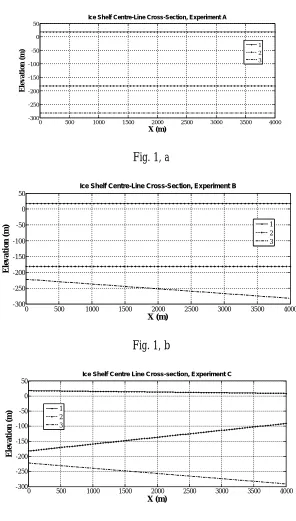
The numerical experiments with ice tongue forced vibrations were carried out for a physically idealized ice plate having rectangular and trapezoidal profiles (Fig. 1).The three experiments that differ in ice tongue/cavity geometries as shown in Fig.1, are considered here. A difference in the spectra obtained between the three experiments implied the impact of the cavity geometry and of the ice tongue geometry, respectively, to the eigen frequencies of ice-water system. In Experiment A ice tongue thickness and the water layer depth were kept constant (Fig. 1, a).
In Experiment B an expanding water layer was considered (Fig. 1, b).The expanding water layer is in agreement with the observations (e.g., Holdsworth and Glynn, 1978)and leads to the change in the velocity of spreading of a long gravity wave in the channel (due to changes of d ). Therefore, the cavity geometry change alters the eigenvalues and, thus, it reflects the impact of the cavity geometry to the eigen frequencies of ice-water system.
In addition, in Experiment C a tapering ice tongue was considered (Fig. 1, c).Likewise, as in the case of the expanding cavity, firstly, the tapering ice tongue is in agreement with the observations (i.e. the shape qualitatively matches observations for a particular ice tongue (Holdsworth and Glynn, 1978)).Secondly, the taper of the ice tongue should yield changes of the eigen frequencies of ice-water system due to change of the average ice-plate thickness.
In this paper the experiments was mainly implemented for relatively high
aspect ratio γ ≈ 0.03 (γ= ). In the case of relatively high aspect ratio γ ≥0.03
the full model yields the spectra that are in a good agreement with theHoldsworth and Glynn model. The experiment A was also implemented for the lower value γ ≅ 0.01, at which we already observe a sufficient distinction in the spectra at a low frequencies.
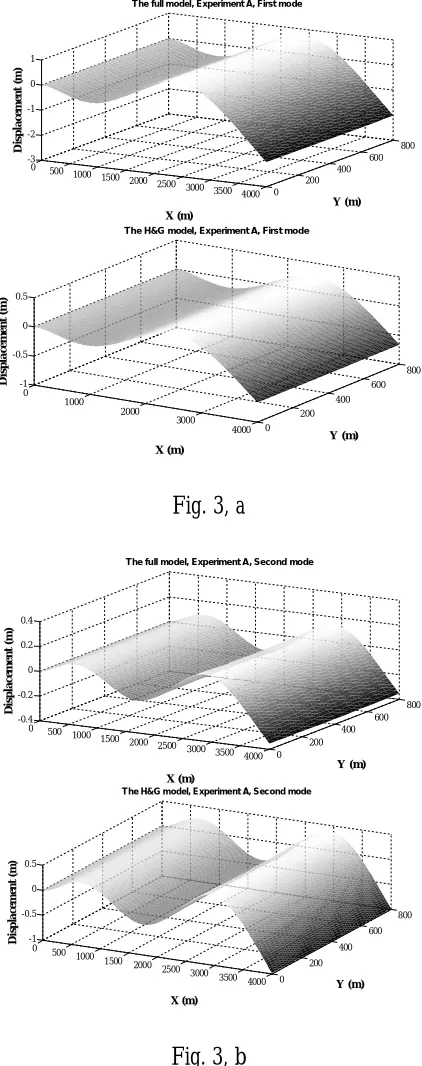
Figure 3, shows the ice tongue deformations that responded to the Eigen frequencies derived from the amplitude spectra in Experiment A.
Fig. 1, a
Fig. 1, b
Fig. 1, c
0 500 1000 1500 2000 2500 3000 3500 4000
-300 -250 -200 -150 -100 -50 0 50
Ice Shelf Centre-Line Cross-Section, Experiment A
X (m) E le v a ti o n ( m
) 12
3
0 500 1000 1500 2000 2500 3000 3500 4000
-300 -250 -200 -150 -100 -50 0 50
Ice Shelf Centre-Line Cross-Section, Experiment B
X (m) E le v a ti o n ( m ) 1 2 3
0 500 1000 1500 2000 2500 3000 3500 4000
-300 -250 -200 -150 -100 -50 0 50
Ice Shelf Centre Line Cross-section, Experiment C
Figure 1: The ice-shelf and the cavity geometries that are considered in the three numerical experiments (A, B, C), respectively.1 – ice-shelf surface, 2 – ice-shelf base, 3 – sea bottom. Aspect ratio γ ≈0.03.
Experiment A. The first four eigen values can be distinguished easily in the spectra shown in Fig. 2 (γ= 0.035). They are approximately equal to 37.1s, 14.2s, 7.1s, 4.21s in the full model and are approximately equal to 41.1s, 14s, 6.7s, 3.81s, respectively, in the Holds worth and Glynn model. The maximum difference between the eigen values is observed for the first eigen value, which corresponds to the largest peak in the spectra in Fig. 2,a. The relative deviation for the first four eigen values varies from 2% to 10%.Although, more careful observation reveals that the models provide different spacing between the resonance peaks. The intervals are smaller in the full model. The deformations obtained by the two models, are in agreement in the spatial distributions of nodes/antinodes (Fig. 3).
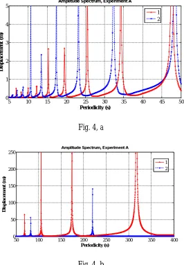
In addition to the considered experiment, where the aspect ratio was taken equal to 0.035, the rectangular ice tongue with the aspect ratioγ = 0.01was considered. The ice tongue has the following geometric parameters: ice thickness is equal to 100 m, sub-ice water depth is equal to 100 m, ice width is equal 300 m, and ice length is equal to 10 km. Figure4 shows the spectrum obtained for the ice tongue with γ= 0.01. In the short-period part of the spectrum (Fig. 4,a) the comparison shows relatively good agreement between the two considered models. Like in the previous experiment, wherein γ = 0.035,the models provide different spacing between the resonance peaks. However, in the long-period part of the spectrum (Fig. 4,b) the significant distinction is observed. The Holdsworth and Glynn model provides only two resonance peaks in the range 50..300 s at T ≈220s and at
T ≈82s, while the full model yields four resonance peaks at T ≈317s; T ≈
Fig. 2, a
Fig. 2, b
Figure 2: The amplitude spectra, maximal ice-shelf deflection versus ocean wave periodicity, obtained in Experiment A (Fig. 1, a). Сurve 1 is the amplitude spectrum derived from the full model. Сurve 2 is the amplitude spectrum obtained by the Holdsworth and Glynn model. The amplitude spectra are obtained at different temporal resolutions: a) temporal resolution is equal to 0.1s for periodicity varying in the range from 5s to 50s; b) temporal resolution is equal to 0.01s for periodicity in the range from 3s to 5s.Aspect ratio γ = 0.035.
5 10 15 20 25 30 35 40 45 50
0 1 2 3 4 5 6
Amplitude Spectrum, Experiment A
Periodicity (s)
D
is
p
la
ce
m
en
t
(m
)
1 2
3 3.2 3.4 3.6 3.8 4 4.2 4.4 4.6 4.8 5
0 0.2 0.4 0.6 0.8 1 1.2 1.4
Amplitude Spectrum, Experiment A
Periodicity (s)
D
is
p
la
ce
m
en
t
(m
)
Fig. 3, a
Fig. 3, b
0 500
1000 1500 2000 2500 3000 3500 4000 0 200 400 600 800 -3 -2 -1 0 1 Y (m) T he full model, Experiment A, First mode
X (m) D is p la ce m en t (m ) 0 1000 2000 3000 4000 0 200 400 600 800 -1 -0.5 0 0.5 Y (m)
The H&G model, Experiment A, First mode
X (m) D is p la ce m e n t (m )
0 500 1000
1500 2000 2500 3000 3500 4000 0 200 400 600 800 -0.4 -0.2 0 0.2 0.4 Y (m) T he full model, Experiment A, Second mode
X (m) D is p la c em e n t (m ) 0 500 1000 1500 2000 2500 3000
3500 4000 0 200 400 600 800 -1 -0.5 0 0.5 Y (m) T he H&G model, Experiment A, Second mode
Fig 3, c
Figure 3.Ice-shelf deformations obtained for the first three modes in Experiment A. Aspect ratio γ= 0.035. The left plots show the deformations obtained by the full model. The right plots show the deformations obtained by the Holdsworth and Glynn model. a) The periodicities are equal to 37.1s and to 41.1s, respectively; b) the periodicities are equal to 14.2 s and to 14 s, respectively; c) the
periodicities are equal to 7.1s and to 6.7s, respectively. Young's modulus E9GPa, Poisson's ratio 0.33 (Schulson, 1999).
0 500 1000 1500 2000 2500 3000 3500 4000 0 200 400 600 800 -0.6 -0.4 -0.2 0 0.2 Y (m) T he full model, E xperiment A, T hird mode
X (m) D is p la ce m en t (m ) 0 500
1000 1500 2000
2500 3000 3500 4000 0 200 400 600 800 -0.15 -0.1 -0.05 0 0.05 Y (m)
The H&G model, Experiment A, Third mode
Fig. 4, a
Fig. 4, b
Figure 4. The amplitude spectra obtained in Experiment A for ice tongue, which has 10 km ice length, 100 m ice thickness and 300 m ice width. Sub-ice water depth is equal to 100 m. Aspect ratio γ= 0.01.Сurve 1 is the amplitude spectrum derived from the full model. Сurve 2 is the amplitude spectrum obtained by the Holdsworth and Glynn model. The amplitude spectra are obtained at different temporal resolutions: a) temporal resolution is equal to 0.1s for periodicity varying in the range from 5s to 50s; b) temporal resolution is equal to 0.2s for periodicity in the range from 50s to 400s.
5 10 15 20 25 30 35 40 45 50
0 1 2 3 4 5
Amplitude Spectrum, Experiment A
Periodicity (s)
D
is
p
la
c
em
en
t
(m
)
1 2
50 100 150 200 250 300 350 400
0 50 100 150 200 250
Amplitude Spectrum, Experiment A
Periodicity (s)
D
is
p
la
c
e
m
e
n
t
(m
)
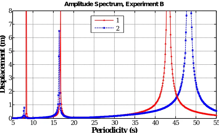
Experiment B. This experiment reveals the same trend in the difference between the eigenvalues obtained from both the considered models (Fig. 5; aspect ratioγ ≈0.03). Specifically, likewise as in Experiment At he maximum difference between the eigenvalues is observed for the first eigenvalue. The first three eigenvalues are approximately equal to 43.2s, 16.8s, 8.4s in the full model and are approximately equal to 48.3s, 16.5s, 7.9s, respectively, in the Holdsworth and Glynn model. The maximum relative deviation is also equal to about 11%. Moreover, Experiment B justified the eigenvalue dependence on the cavity geometry in both the considered models. The deviation for the eigenvalues due to the cavity geometry changes is about 17% (Tab. 1).
Table 1: Eigen value difference due to cavity geometry changes and due to ice-shelf geometry changes in the full model
Eigenvalue T T T
Experiment A
3 7.1
14. 2
7. 1
Experiment B
4 3.2
16. 8
8. 4
Experiment C
6 6.9
21. 2
1 0.3 Deviation (B
vs. A)
1 5%
17 %
1 7% Deviation (C
vs. A)
5 7%
40 %
Figure 5.The amplitude spectra obtained in Experiment B (Fig. 1, b). The red curve is the amplitude spectrum obtained by the full model. The blue curve is the amplitude spectrum obtained by the Holdsworth and Glynn model. Aspect ratioγ ≈
0.03.
Experiment C. There are no new particulars (in comparison with previous experiments) in the relative position of the resonance peaks obtained from the considered models (Fig. 6) in Experiment C (for aspect ratio γ ≈ 0.03). The first four eigen values are approximately equal to 66.9s, 21.2s, 10.3s, 5.9s in the full model and are approximately equal to 68.8s, 20.5s, 9.8s, 5.5s, respectively, in the Holds worth and Glynn model. The maximum relative deviation for the tapering ice tongue is smaller in comparison with the previous values (in Experiment A and B) and is about 3..7%. Experiment C in comparison with Experiment B similarly shows that the ice tongue geometry change (average ice tongue thickness increase/decrease) also yields shifts in the resonance peaks. The relative deviation due to the ice tongue geometry change is about 37% to 57% (Tab. 1). Likewise as in Experiment A, for corresponding eigen values the deformations are in agreement for the two considered models.
5 10 15 20 25 30 35 40 45 50 55
0 1 2 3 4 5 6 7 8
Amplitude Spectrum, Experiment B
Periodicity (s)
D
is
p
la
ce
m
e
n
t
(m
)
Figure 6.The amplitude spectra obtained in Experiment C (Fig. 1, c). The red curve is the amplitude spectrum obtained by the full model. The blue curve is the amplitude spectrum obtained by the Holdsworth and Glynn model. The temporal resolution is equal to 0.1s. Aspect ratio γ ≈0.03.
4. Conclusions
The numerical experiments have shown the impact of tongue/cavity geometry on the amplitude spectrum. The alterations of the geometries excite shifts in the peak positions. Therefore, the ability of prediction of resonant-like icetongue/shelf motion requires accounting for (i) detailed ice-shelf surface/base topography (ii) detailed numbers and positions of the crevasses, and (iii) detailed seafloor topography under the ice-shelf.
The full 3D model yields quantitatively similar results, which were obtained by a model based on thin-plate approximation (Holdsworth and Glynn, 1978) for relatively high aspect ratio (here γ ≈0.03 was considered). The maximum relative deviation for the eigenvalues in the test experiments does not exceed 11% and the maximum is observed for the first eigenvalue. Vice versa, there is significant distinction in the long-period part of the spectra for smaller values of the aspect ratio, in particular, for γ= 0.01.
0 10 20 30 40 50 60 70 80 90
0 5 10 15
Amplitude Spectrum, Experiment C
Periodicity (s)
D
is
p
la
ce
m
en
t
(m
)
The difference appears in the eigenvalues and in the number of the resonance peaks. Thus, the Holdsworth and Glynn model doesn’t confirm the spectra generated by the full model for the smaller aspect ratio γ< 0.01.The explanation of the difference can be suggested from the mathematical point of view, considering the eigenvalues as the roots of the equation D(ω) = 0, in which D(ω) is the determinant of the matrix resulted from discretization of the model.
The determinant D(ω) is a bi-polinomial expression and his roots depend on the number of equations of the model. Since the thin plate approximation suggests reduction of the number of equations in comparison with the full model (supposing that σ =σ = σ ≈0 in the plate), so we can anticipate the decline of the set of roots and, therefore, the decrease of the array of eigenvalues in the approximated model. Essentially, this reduction is observed in the obtained spectra: in the considered experiments (a) for γ ≈0.03the observed smaller spacing between resonance peaks in the full model (for instance, Fig.2) implies the increasing of the set of the peaks in the full model spectra and (b) for γ= 0.01 the increasinghas explicitly appeared in the considered parts of the full model spectrum (Fig. 4).
Appendix A: Field equations of the thin-plate model (Houlds worth & Glynn model)
Houlds worth & Glynn forced vibration model (1978), which is considered in the test experiments (A, B and C) as the basic model, includes following equations.
Thin-plate vibration equation (the momentum equation) is
+ −2 =ρ H + ρ gW−P ; (A1)
whereW(x, y, t) is vertical deflection;ρ is ice density;His ice-shelf thickness; ρ isseawater density;g is the acceleration of gravity;P′ is the deviation from the hydrostatic pressure;M , M , M are bending moments to lateral loading and they are expressed as
M =−D + ν ; (A3)
M = D(1− ν) ; (A4)
whereDis flexural rigidity: D =
( ).
The wave equation for water layer is
= d + d ; (A5)
whered (x, y) is the depth of the sub-ice water layer.
The boundary conditions are
At x = 0 (fixed boundary): W = 0; = 0; M = M ;
M = 0; = 0.
At x = L (ice-shelf terminus): M = 0; M = D ; =
2 ; M = D(1− ν) ; P = Aρ g sinωt; where A is the
amplitude of the incident wave, ω is the frequency of the forcing (incident wave).
At y = 0, y = L (lateral edges of the ice-shelf): M = 0; M =
D ; = 2 ; M = D(1− ν) ; = 0.
Appendix B: Boundary conditions employed in the full model
We rewrite, for instance, the first equation from (1) using the new variables:
+η +ξ′ + η +ξ + ξ′ = ρ .
We write the approximation of the derivative at the ice-shelf base
towards the substance (glacier):
ξ′ = − ≈ − σ + σ − σ ;
Where index "N " corresponds to grid layer located at the ice shelf base.
The standard (typical) boundary condition at the ice-shelf base (3) requires
thatσ = σ +σ + P . Thus, we should replace σ in agreement with
the standard boundary conditions, with σ +σ + P . Finally, we
obtain the following approximation of the derivative ξ′ at the ice-shelf base:
ξ ≈ − σ + σ − σ +
σ − P − ρg ;
where P =ρgH + P′.
Thus, at the ice shelf base, we apply the equation
+ η + ξ′ + η + ξ −
σ + + σ − σ +σ − P ≈
Which is the first equation at the ice-shelf base, instead of the standard
equation σ = σ +σ + P .
Therefore, after the coordinate transformation, the applicable equations at ice-shelf base can be written as
⎩ ⎪ ⎪ ⎪ ⎪ ⎪ ⎪ ⎪ ⎨ ⎪ ⎪ ⎪ ⎪ ⎪ ⎪ ⎪
⎧ + η + ξ′ + η + ξ − σ +
σ − σ +σ − P ≈ ρg +ρ ;
+ η + ξ′ + η + ξ − σ +
σ − σ +σ − P ≈ ρg +ρ ;
+ η + ξ′ + η + ξ − σ +
σ − σ +σ + P ≈ − ρg +ρg +ρ .
(B1)
The same method yields the similar equations at the ice surface
⎩ ⎪ ⎪ ⎪ ⎪ ⎪ ⎪ ⎪ ⎨ ⎪ ⎪ ⎪ ⎪ ⎪ ⎪ ⎪
⎧ + η + ξ′ + η + ξ +
σ +σ − σ + σ ≈ ρ ;
+ η + ξ′ + η + ξ +
σ +σ − σ + σ ≈ ρ ;
+ η + ξ′ + η + ξ +
σ +σ − σ + σ ≈ ρg +ρ ;
where indices, "1", "2", "3", denote respectively the numbers of the grid layers starting from the ice surface to moving downward in the vertical direction.
Finally, the same manipulations lead to the following equations at the free edges:
At x = L:
⎩ ⎪ ⎪ ⎨ ⎪ ⎪
⎧ σ − σ ≈ − f(ξ)− ξ ( )+ρ ;
σ − σ + η + ξ + ξ′ ≈ ρ ;
σ − σ + η + ξ + ξ′ ≈ ρg +ρ ;
(B3)
wheref(ξ) = 0, ξ< ;
ρ g(h − ξH), ξ ≥ .
At y = y (x):
⎩ ⎪ ⎪ ⎪ ⎪ ⎪ ⎪ ⎪ ⎪ ⎪ ⎨ ⎪ ⎪ ⎪ ⎪ ⎪ ⎪ ⎪ ⎪ ⎪
⎧ + η + ξ′ − η σ + η σ −
η σ + ξ + ξ ≈
≈ − η f (ξ) + ξ +ρ ;
+ η + ξ′ − η σ + η σ −
η σ + ξ + ξ ≈
≈ − η f (ξ) + ξ +ρ ;
+ η + ξ′ − η σ + η σ −
η σ + ξ + ξ ≈ ρg +ρ ;
where indices, "1", "2", "3", denote respectively the numbers of the grid layers starting from the ice lateral edge y = y (x), moving in the horizontal transverse direction in the glacier; and
f = 0, ξ< ;
ρ g(h − ξH) , ξ ≥ .
f = 0, ξ< ;
−ρ g(h − ξH), ξ ≥ .
At y = y (x):
⎩ ⎪ ⎪ ⎪ ⎪ ⎪ ⎪ ⎪ ⎪ ⎪ ⎪ ⎨ ⎪ ⎪ ⎪ ⎪ ⎪ ⎪ ⎪ ⎪ ⎪ ⎪
⎧ + η + ξ′ + η σ −
η σ + η σ + ξ + ξ ≈
≈ − η f (ξ)− ξ +ρ ;
+ η + ξ′ + η σ −
η σ + η σ + ξ + ξ ≈
≈ − η f (ξ)− ξ +ρ ;
+ η + ξ′ + η σ −
η σ + η σ + ξ + ξ ≈
≈ ρg +ρ ;
(B5)
f = 0, ξ< ;
−ρ g(h − ξH) , ξ ≥ .
f = 0, ξ < ;
ρ g(h − ξH), ξ ≥ .
Acknowledgements
The author is grateful to Dr. E. Bueler for useful comments to the manuscript.
References
Bassis, J.N., Fricker,H.A., Coleman,R., Minster,J.-B. (2008).An investigation into the forces that drive ice-shelf rift propagation on the Amery Ice Shelf, East Antarcyica.J. of Glaciol.; 54 (184), 17-27.
Bromirski, P.D., Sergienko, O.V., MacAyeal, D.R. (2009). Transoceanic infragravity waves impacting Antarctic ice shelves. Geophys. Res. Lett., 37, L02502, doi:10.1029/2009GL041488.
Goodman, D.J., Wadhams,P.& Squire,V.A. (1980)The flexural response of a tabular ice island to ocean swell. Ann. Glaciol., 1, 23–27.
Holdsworth, G. (1977).Tidal interaction with ice shelves. Ann. Geophys., 33, 133-146.
Holdsworth, G. & Glynn,J. (1978) Iceberg calving from floating glaciers by a vibrating mechanism. Nature, 274, 464-466.
Hughes, T. J. (1977). West Antarctic ice streams. Reviews of Geophysics and Space Physics,15(1), 1-46.
Konovalov, Y.V. (2012).Inversion for basal friction coefficients with a two-dimensional flow line model using Tikhonov regularization. Research in Geophysics, 2:e11, 82-89. Konovalov, Y.V. (2014).Ice-shelf resonance deflections modelled with a 2D elastic centre-line
model. Physical Review & Research International, 4(1), 9-29.
Lamb, H.(1994).Hydrodynamics.(6th ed.).Cambridge: Cambridge University Press.
Landau, L.D., Lifshitz, E.M. (1986). Theory of Elasticity.(3rd ed.).Oxford:Butterworth-Heinemann,(Vol. 7).
Lingle, C. S., Hughes, T. J., & Kollmeyer, R. C. (1981).Tidal flexure of Jakobshavns Glacier, West Greenland. J. Geophys. Res.,86(B5), 3960- 3968.
MacAyeal, D.R., Okal,E.A., Aster,R.C., Bassis,J.N., Brunt,K.M., Cathles, L.M., Drucker, R., Fricker, H.A., Kim, Y.-J., Martin,S., Okal, M.H., Sergienko, O.V., Sponsler, M.P., & Thom,J.E.(2006). Transoceanic wave propagation links iceberg calving margins of Antarctica with storms in tropics and Northern Hemisphere. Geophys. Res. Lett., 33, L17502, doi:10.1029/2006GL027235.
Meylan M., Squire, V.A., & Fox,C. (1997).Towards realism in modelling ocean wave behavior in marginal ice zones.J. Geophys. Res., 102(C10), 22981–22991.
Reeh, N., Christensen, E.L., Mayer, C., Olesen, O.B. (2003). Tidal bending of glaciers: a linear viscoelastic approach. Ann. Glaciol., 37, 83–89.
Robin, G. de Q. (1958).Seismic shooting and related investigations. In: Norwegian-British-Swedish Antarctic Expedition, Sci. Results 5, Glaciology 3,NorskPoarinstitutt (pp. 1949-1952). Oslo: University Press.
Rosier, S.H.R., Gudmundsson, G.H., & Green, J.A.M. (2014). Insights into ice stream dynamics through modeling their response to tidal forcing. The Cryosphere, 8, 1763– 1775.
Schmeltz, M., Rignot, E., & MacAyealD.R. (2001). Tidal flexure along ice-sheets margins: Comparison of InSAR with an elastic plate model. Ann. Glaciol., 34, 202-208. Schulson, E.M. (1999).The Structure and Mechanical Behavior of Ice.JOM, 51 (2), 21-27. Sergienko, O.V. (2010).Elastic response of floating glacier ice to impact of long-period ocean
waves. J. Geophys. Res., 115, F04028, doi:10.1029/2010JF001721.
Smith, A.M. (1991).The use of tilt meters to study the dynamics of Antarctic ice shelf grounding lines. J. Glaciol., 37, 51–58.
Squire, V.A., Dugan, J. P., Wadhams, P., Rottier, P. J.,& Liu,A.K. (1995).Of ocean waves and sea ice. Annu. Rev. Fluid Mech., 27, 115–168.
Stephenson, S.N. (1984). Glacier flexure and the position of grounding lines: measurements by tilt meter on Rutford Ice Stream, Antarctica. Ann. Glaciol., 5, 165-169.
Turcotte, D.L.,& Schubert,G. (2002).Geodynamics.(3rd ed.).Cambridge: Cambridge University Press.
Vaughan, D.G. (2002).Tidal flexure at ice shelf margins. J. Geophys. Res., 100(B4), 6213-6224.
Wadhams, P. (1986).The seasonal ice zone. In Untersteiner, N.(Ed.), Geophysics of sea ice (pp. 825–991). London: Plenum Press.