Dynamical Process On Growing Geometrical Network Based
On Modular Group
N. N. A. Kamal1, K. T. Chan1,2*, N.M. Shah1,2, and H. Zainuddin1,2
1Laboratory of Computational Sciences and Mathematical Physics, Institute for
Mathematical Research (INSPEM), Universiti Putra Malaysia, Malaysia 2Department of Physics, Faculty of Science, Universiti Putra Malaysia, 43400 UPM
Serdang, Selangor, Malaysia
∗Corresponding author: [email protected]
Many network models have been proposed and constructed to mimic the underlying features of complex networks. Studying the dynamical process of a network gives a good platform to understand how the underlying geometrical and structural features influence various transport properties. In this study, the dynamical process on the network is described by using random walks. From this process, some of the random walk transport properties are determined such as relaxation time, mean first passage time (MFPT), random walk centrality (RWC), average trapping time (ATT) and global mean first passage time (GMFPT). We find that GMFPT grows exponentially when the network grows. This is mainly due to some central nodes that have high RWC, which tends to attract the random walker more compared to a node with a lower RWC. This study plays an important role in determining the performance of the network.
Keywords: Complex networks, Mean first passage time, Random walk, Random walk centrality
I.
Introduction
The world is abundant of complex networks in various field from biology, physics to computer science. One of the earliest network models is introduced by Watts and Strogatz (1998) which shows that most of the real-world networks ex-hibit features like small-world network that has high clustering coefficient. Another type of net-work model is scale-free (SF) netnet-work based on Albert et al. (1999) that follows power-law degree distribution Pdeg(K) ∼ K(−γ) where
Pdeg(K) is the fraction of nodes with the
num-ber of links attached to it known as degree,K. To have a scale-free property, usually the power law exponent, γ is at the range of 2 6γ 63. SF network is an example of heterogeneous network and it has significant effect on phys-ical problems where it is stable in opposition to the removal of nodes but fragile under
broadly are relaxation time (τ), mean first pas-sage time (MFPT) from one node to another node and the random walk centrality (RWC).
MFPT,hTijiis defined as the time needed for
a walker to reach a node from a starting point and this property is widely used in character-izing transport efficiency (Kozak and Balakr-ishnan, 2002, Zhang et al., 2009, 2010) It was shown that MFPT behaves differently depend-ing on the topology. For example, it behaves sublinearly with the size of network,N in some scale-free networks while behaves very differ-ently in standard regular fractals (Bentz et al., 2010, Lin et al., 2010) where it scales superlin-early with N. MFPT plays an important role in determining the RWC which describes cen-tralization of information travelling over net-works and also the average trapping time hTji,
which is the average of MFPT to the trap node j taken over all starting point. Besides, with the calculation of MFPT, global mean first pas-sage time (GMFPT) for the whole network can also be determined.
In this paper, we compute MFPT on a grow-ing geometrical network (GGN) constructed from tessellation of modular group (Taha et al., 2016). Based on the calculated MFPT value, we can explain how the walker behaves in GGN via the study of transport properties such as RWC, relaxation time, ATT as well as GMFPT. Besides, by studying these transport properties, we can shed some light about the structure of the network either it being a ho-mogeneous or a heterogeneous network.
A. Random Walks on Network
To apply the RW, first, we consider the GGN network, represented as G(V, E) where V is the set of nodes while E is the set of undi-rected edges. The connection of two nodes i and j can be represented by adjacency matrix,
A which equals to 1 if there is a relation be-tween them and 0 if otherwise. Since the GGN is an undirected network, it has the property of Aij = Aji. For degree of node i, it is given
as Ki = PjAij . As for the walker, since it
cannot remain at the same node, it will move
to another node once at a time with the prob-ability of K1
i. Using the adjacency matrix and the probability, we can determine the transi-tion probability which is defined by the walker movements. If the walker is on node iat time tchooses one of its neighbour with equal prob-ability at timet+ 1, the transition probability can be written asWij = AKiji . Since the walker
starts at node i at time t = 0 and arrived at node j at time t; the master equation can be expressed as
Pij(t+ 1) = X
k
Akj
Kk
Pik(t). (1)
Since there is no boundary in network, the ran-dom walker can move in any direction inside the GGN. However, it cannot leave the system and this is similar to the diffusion process ex-cept that all walkers must follow the equation at every time step (Lau and Szeto, 2010). In order to find the walker probability atj fromi att, the asymptotic behaviour of the transition probability is considered. Based on the princi-ple of detailed balance with t→ ∞, the system reaches a state where there is no net flow of random walker in any direction. This leads to KiPj∞=KjPi∞ where
Pj∞= lim
t→∞Pij(t).
The equilibrium state can be defined as
Pj∞= Kj
2L. (2)
where L denotes the number of edges. Based on Eq.2 at equilibrium state, the walker has a higher tendency to move to nodes with more edges. In the other hand if the system’s net flow is not zero, it will consist of both equilibrium state probability and fluctuation around it.
In order to figure out the MFPT, we need to find a relation between first passage time, Fij(t) and probability of the walker to reach
the destination,Pij(t). This relation described
at t, then returns to j after t−t0 steps (Red-ner, 2001). Thus, the first-passage probability satisfies the relation
Pij(t) =δijδt0+
t X
t0−0
Fij(t)Pjj(t−t0). (3)
where δijδt0 represents to the initial condition of the walker probability. This equation can be decoupled by using Laplace transform (Hughes, 1995, Redner, 2001) and yields
˜
Pij(s) =δij + ˜(F)ij(s) ˜Pjj(s). (4)
The details of the formulation of MFPT are explained in Samsul et al. (2018). By express-ing the terms in Eq.4 with Laplace transform, MFPT, hTiji is obtained as follows
hTiji= 2L Kj h
R(0)jj −Rij(0)i forj6=i
2L
Kj forj=i
(5)
Other than MFPT, another transport prop-erty of random walk that can be identified here is the relaxation time, τ where it is the asymp-totic time of convergence to the equilibrium or stationary distribution. It is defined as
τj =R(jjn)≡
∞
X
t=0
Pjj(t)−Pj∞
. (6)
Another measurement called random walk centrality can also be obtained when the ran-dom walk motions are asymmetric, i6=j. The measurement equation is given by
Cj ≡
Pj∞ τj
. (7)
It measures the speed of the walker to move from one node to another node. The walker will reach the target node earlier in consequence of high RWC value. This property plays different effects depending on the type of network. For example, in terms of communication, a node with high RWC will receive signal emitted by its partner earlier (Noh and Rieger, 2004). Us-ing the MFPT computed from Eq.5, we can
study the trapping problem defined on GGN. Let hTji be the average trapping time, or the
average of MFPT, hTiji to the trap node j,
taken over all starting point. The equationhTji
is expressed as
hTji=
1 N −1
N X
j=1
hTiji − hTiii
. (8)
For the GMFPT, hTgi, it is defined as average
over all the trap nodes for the network. The formulation of hTgi is expressed by
hTgi=
hTji
N . (9)
II.
Methodology
The growing geometrical network in this study is constructed based on using modular group, a discrete subgroup of P SL(2, R) tessellating the hyperbolic plane. The tessellation is gen-erated with Mathematica by using linear frac-tional transformation and can be found in Taha et al. (2016). As number of iterations increases, the size of the network grows exponentially pro-ducing large number of nodes and edges. This is due to the growth of concatenation of words or generators of the modular group (Taha et al., 2016). Table 1 shows the total number of nodes and edges produced from different itera-tion while Figure 1 shows the constructed net-work.
To compute the value of MFPT based on Eq.5, a matrix formulation needs to be formed first by using equation Rnij ≡ P∞
t=0[Pij(t) − Pj∞]. The equation can be written as
R(0) =
∞
X
t=0
(Wt−Q). (10)
where R(0) is similar to Rij(0). Matrix W
in Eq.10 represents the transition matrix and
Q≡P∞1 represents the equilibrium probabil-ity matrix. A relation ofQn=Qforn >0 and
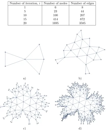
Table 1: Total number of nodes and edges produced from different iteration.
Number of iteration, i Number of nodes Number of edges
1 6 8
5 23 44
10 100 207
15 414 872
20 1695 3585
a) b)
c) d)
Figure 1: Underlying network from the modular group tessellation with iteration a)i = 1, b)i= 5, c)i= 10 and d)i= 15
.
subspace with eigenvalue 1 (Noh, 2007). From these relations,Wn−Q= (W−Q)nforn >0
and (I−Q) for n = 0. Applying all of them into Eq.10, it can be redefined as
R0= 1
I+Q−W −Q. (11)
To determine both MFPT and RWC, Eq.11
III.
Results and Discussion
Computation of MFPT has been carried out on networks constructed from tessellation of mod-ular group on a hyperbolic plane with different sizes. Computing MFPT enables us to know what is the mean time for a random walker to reach a particular node for the first time. With the MFPT values for every node in a particular network, we can compute the average trapping time (ATT), hTji for a particular trap node j
taken over all starting points in the network. ATT is important as it can be used to charac-terize the network structural properties based on transport efficiency. One example of trap-ping problem is the work of Montroll (1969) in the application to excition trapping on photo-synthesis units.
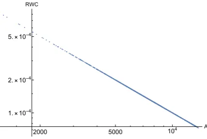
2000 5000 104 ATT
1.×10-4
2.×10-4
5.×10-4 RWC
Figure 2: Log-log plot of random walk central-ity vs average trapping time for modular group at 20th iteration.
Figure 2 shows the graph plot of RWC against the ATT for every node in 20th it-eration GGN. Table 1 shows the number of nodes increases as the iteration, i increases. i = 1,5,10,15,20 are chosen generally to re-flect on how the network grows. However, we generate the network model for each iteration between 1 ≤ i ≤ 20. According to Table 1, a 20th iteration GGN has 1695 nodes and 3585 number of edges. RWC is decreasing linearly with the ATT which implies that the longer the time needed for the walker to arrive at cer-tain nodes, the less important that the node becomes in the network. For example, a less
important node in the network will be less vis-ited by the walker in comparison to the other nodes. Say we have two nodes where Cj > Ci,
the random walker that starts at node i will reachj earlier compared to when it started on nodejand wants to reach i. Thus a node with a larger RWC tends to be visited earlier by the random walker rather than a node with smaller RWC. In another word, a node with a high val-uer of RWC will attract the walker to visit it more frequently. Also, a high value of RWC in a node indicates that the node is important in diffusion or trapping process.
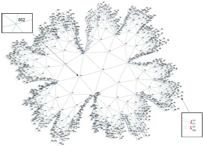
Structure of the network plays an important role in determining the values of RWC and ATT for a particular node. In Tables 2 and 3, we identify the highest and lowest ten values of ATT and RWC for nodes in the GGN. The location of these nodes is also highlighted in the network as shown in Figure 3. Nodes with the highest values of ATT (red in colour) are all located at the periphery part of the network. On the other hand, nodes with lowest values of ATT (green in colour) are all located at the center of the network. This shows that the cen-tral part of the network or the ”freeze” region has the most effective communication between nodes while the outer regions are pretty much less effective.
If we look at the degree of the nodes on the network, they are distributed between the range of 2 ≤ K ≤ 18. Nodes with the high-est values of ATT are all having value of K = 2. Meanwhile, the nodes with lowest values of ATT possess the value of K ranging from 6 ≤ K ≤ 18. From the static process, by looking at the degree distribution, the network can be identified as a heterogeneous network because the degree is not distributed evenly. From the dynamical process, RWC or ATT val-ues can be used to explain this matter as their distribution shows asymmetry in the network.
Figure 3: GGN at 20th iterations where the magnified points show the highest and the lowest values of ATT.
Table 2: Lowest values of ATT.
Nodes ATT RWC K
661 1280.41 0.000783507 18 3 1335.20 0.000750921 18 288 1539.2 0.000651432 17 289 1558.59 0.000643515 6 662 1655.63 0.000605669 6 424 1824.68 0.000549441 6 1119 1832.4 0.000546916 17
128 1913.76 0.000523787 6 975 2049.37 0.00048903 6 974 2078.804 0.000482091 6
K. A short relaxation time in random walk is known as random walks with non-compact ex-ploration (B´enichou et al., 2010, Hwang et al.,
Table 3: Highest values of ATT.
Nodes ATT RWC K
739,740 13687.5 0.00007308 2 602,603 13569.9 0.000073714 2 569,570 13534.5 0.0000739081 2 561,562 13475.7 0.0000742325 2 332,333 13363.4 0.0000748545 2
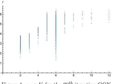
2 4 6 8 10 12 K 1
2 3 4 5 6
τ
Figure 4: τ vsK for the 20th iteration GGN.
degree of six. This is because node with degree six is usually nodes that form the central part (saturated part) of the network and they ap-peared the most in the network. These nodes are not only appeared at the central region, they also appeared in different region of the network. Hence, the relaxation time turns out to be distributed broadly between 1 ≤τ ≤7. On the contrary, another region with different value of K has much smaller range of τ due to active boundary of the network (Wu et al., 2015) where it can still link many triangles.
According to Eq.7, τ is inversely propor-tional to RWC. When RWC is high, the re-laxation for that particular node is low. This implies that most nodes in the central regions have low relaxation time which means that they can converge to stationary distribution easily. If we consider the walker as information, it would mean that the information can be sup-plied to all nodes in that region in a short time.
5 10 15 20
Iteration 50
100 500 1000 5000 104
GMFPT
Figure 5: GMFPT vs Iteration.
Then, we compute the GMFPT of every other iteration from the modular group. Figure 5 shows a semi-log plot between GMFPT and iterations and it shows that GMFPT grows ex-ponentially. This trend indicates that it has a power-law function. The linear scaling of GMFPT with the iteration also shows that the underlying structure of the network is het-erogeneous and not homogeneous. This trend can also be observed in complete graphs (Bollt and ben Avraham, 2005). For having hetero-geneous structures, this means that there are central nodes that gas very large degree. These nodes usually have high RWC and the walkers are attracted to them.
High value of GMFPT indicates a longer time for the walker to cover the whole net-work, thus affects the efficiency of the network model. However, when compared to a homoge-neous network (random network), the GMFPT is much lower.
IV.
Conclusion
In summary, we have discussed five transport properties of random walk process in grow-ing geometrical network. From the computed MFPT, we managed to determine the relax-ation time,τ, random walk centrality, average trapping time and global mean first passage time. RWC and ATT have revealed that GGN of interest has heterogeneous structure due to asymmetry in dynamics. As for the relaxation time, we found that the central part (saturated part) of the network has the lowest value. This implies that the central regions have a fast con-verging time. From the global perspective, the linear scaling of GMFPT indicates the struc-ture of the networks has a scale-free property.
Acknowledgments
References
[1] R´eka Albert, Hawoong Jeong, and Albert-L´aszl´o Barab´asi. Internet: Diam-eter of the world-wide web. nature, 401 (6749):130, 1999.
[2] Tomaso Aste, Tiziana Di Matteo, and ST Hyde. Complex networks on hyper-bolic surfaces. Physica A: Statistical
Me-chanics and its Applications, 346(1-2):
20–26, 2005.
[3] O B´enichou, C Chevalier, J Klafter, B Meyer, and R Voituriez. Geometry-controlled kinetics. Nature chemistry, 2 (6):472, 2010.
[4] Jonathan L Bentz, John W Turner, and John J Kozak. Analytic expression for the mean time to absorption for a ran-dom walker on the sierpinski gasket. ii. the eigenvalue spectrum.Physical Review E, 82(1):011137, 2010.
[5] Erik M Bollt and Daniel ben Avraham. What is special about diffusion on scale-free nets? New Journal of Physics, 7(1): 26, 2005.
[6] Reuven Cohen, Keren Erez, Daniel Ben-Avraham, and Shlomo Havlin. Re-silience of the internet to random break-downs. Physical review letters, 85(21): 4626, 2000.
[7] Eugene F Fama. Random walks in stock market prices. Financial analysts jour-nal, 51(1):75–80, 1995.
[8] Barry D Hughes. Random walks and ran-dom environments. 1995.
[9] S Hwang, D-S Lee, and B Kahng. First passage time for random walks in hetero-geneous networks.Physical review letters, 109(8):088701, 2012.
[10] John J Kozak and V Balakrishnan. Ana-lytic expression for the mean time to ab-sorption for a random walker on the
sier-pinski gasket. Physical Review E, 65(2): 021105, 2002.
[11] Hon Wai Lau and Kwok Yip Szeto. Asymptotic analysis of first passage time in complex networks. EPL (Europhysics
Letters), 90(4):40005, 2010.
[12] Zhuo Qi Lee, Wen-Jing Hsu, and Miao Lin. Estimating mean first passage time of biased random walks with short relax-ation time on complex networks. PloS one, 9(4):e93348, 2014.
[13] Yuan Lin, Bin Wu, and Zhongzhi Zhang. Determining mean first-passage time on a class of treelike regular fractals. Physical
Review E, 82(3):031140, 2010.
[14] Elliott W Montroll. Random walks on lattices. iii. calculation of first-passage times with application to exciton trap-ping on photosynthetic units. Journal
of Mathematical Physics, 10(4):753–765,
1969.
[15] Jae Dong Noh and Heiko Rieger. Ran-dom walks on complex networks.
Physi-cal review letters, 92(11):118701, 2004.
[16] Sidney Redner. A guide to first-passage
processes. Cambridge University Press,
2001.
[17] Kamal Nurul Nasha Amalina Samsul, Kar Tim Chan, Shah Nurisya Mohd, and Hishamuddin Zainuddin. First Passage Time Problem on Growing Geometrical
Network, chapter 2, pages 16–23. UPM
Press, 2018.
[18] M. H. M Taha, Kar Tim Chan, and Hishamuddin Zainuddin. Construction of network based on modular group. Jour-nal of Solid State Science and Technology
Letters, (17):93, 2016.
[20] Isuri Wijesundera, Malka N Halgamuge, Thrishantha Nanayakkara, and Thas Nir-malathas. Natural Disasters, When Will
They Reach Me? Springer, 2016.
[21] Zhihao Wu, Giulia Menichetti, Christoph Rahmede, and Ginestra Bianconi. Emer-gent complex network geometry.
Scien-tific reports, 5:10073, 2015.
[22] Zhongzhi Zhang, Yi Qi, Shuigeng Zhou, Wenlei Xie, and Jihong Guan. Exact solution for mean first-passage time on a pseudofractal scale-free web. Physical
Review E, 79(2):021127, 2009.