www.the-cryosphere.net/11/857/2017/ doi:10.5194/tc-11-857-2017
© Author(s) 2017. CC Attribution 3.0 License.
Mapping snow depth within a tundra ecosystem using multiscale
observations and Bayesian methods
Haruko M. Wainwright1, Anna K. Liljedahl2, Baptiste Dafflon1, Craig Ulrich1, John E. Peterson1, Alessio Gusmeroli3, and Susan S. Hubbard1
1Earth Sciences Division, Lawrence Berkeley National Laboratory, 1 Cyclotron Road, MS 74R-316C, Berkeley, CA 94720-8126, USA
2Water and Environmental Research Center, University of Alaska Fairbanks, 306 Tanana Loop, Fairbanks, AK 99775-5860, USA
3International Arctic Research Center, University of Alaska Fairbanks, Fairbanks, AK, USA
Correspondence to:Haruko M. Wainwright ([email protected]) Received: 2 July 2016 – Discussion started: 30 August 2016
Revised: 10 February 2017 – Accepted: 20 February 2017 – Published: 3 April 2017
Abstract. This paper compares and integrates different strategies to characterize the variability of end-of-winter snow depth and its relationship to topography in ice-wedge polygon tundra of Arctic Alaska. Snow depth was measured using in situ snow depth probes and estimated using ground-penetrating radar (GPR) surveys and the photogrammetric detection and ranging (phodar) technique with an unmanned aerial system (UAS). We found that GPR data provided high-precision estimates of snow depth (RMSE =2.9 cm), with a spatial sampling of 10 cm along transects. Phodar-based approaches provided snow depth estimates in a less labori-ous manner compared to GPR and probing, while yielding a high precision (RMSE=6.0 cm) and a fine spatial sampling (4 cm×4 cm). We then investigated the spatial variability of snow depth and its correlation to micro- and macrotopogra-phy using the snow-free lidar digital elevation map (DEM) and the wavelet approach. We found that the end-of-winter snow depth was highly variable over short (several meter) distances, and the variability was correlated with microto-pography. Microtopographic lows (i.e., troughs and centers of low-centered polygons) were filled in with snow, which resulted in a smooth and even snow surface following macro-topography. We developed and implemented a Bayesian ap-proach to integrate the snow-free lidar DEM and multiscale measurements (probe and GPR) as well as the topographic correlation for estimating snow depth over the landscape. Our approach led to high-precision estimates of snow depth (RMSE=6.0 cm), at 0.5 m resolution and over the lidar do-main (750 m×700 m).
1 Introduction
Snow plays a critical role in ecosystem functioning of the Arctic tundra environment through its impacts on soil hy-drothermal processes and energy exchange (e.g., Callaghan et al., 2011). Snow insulates the ground from intense cold during the Arctic winter, limiting the heat transfer between the air and the ground (Zhang, 2005). Snow depth affects ac-tive layer and permafrost temperatures throughout the year (Gamon et al., 2012; Stieglitz et al., 2003), and increased snow depth has resulted in permafrost degradation (Os-terkamp, 2007). Snow’s insulating capacity enhances con-ditions for active soil microbial processes and CO2/CH4 production during the winter (Nobrega and Grogan, 2007; Schimel et al., 2004; Clein and Schimel, 1995; Jansson and Ta¸s, 2014; Zona et al., 2016). In addition, snow serves as an important water source to tundra ecosystems during the growing season and therefore has a large impact on bio-logical processes via hydrology. Snowmelt water can lead to extensive inundation of low-gradient tundra and large runoff events in early summer (Bowling et al., 2003; Kane et al., 1991; Liljedahl et al., 2016). Since soil biogeochemistry and vegetation are controlled by soil moisture (Sjögersten et al., 2006; Wainwright et al., 2015), the amount of snow af-fects ecosystem functioning throughout the season.
the high Arctic (Zona et al., 2011). The ice wedges de-velop when frost cracks occur in the ground, and vertical ice wedges grow laterally over years (Leffingwell, 1915; MacKay, 2000). Soil movement associated with ice-wedge development creates small-scale topographic variations – mi-crotopography– where the ground surface elevation can vary significantly over lateral length distances of several meters (e.g., Brown, 1967; MacKay, 2000; Engstrom et al., 2005; Zona et al., 2011). This microtopography leads to dramat-ically variable snow depth across short distances. Liljedahl et al. (2016) found that the differential snow distribution in-creased the partitioning of snowmelt water into runoff, lead-ing to less water stored on the tundra landscape. Gamon et al. (2012) reported that snow depth heterogeneity results in differential thawing and active layer thickness variability. In addition, there is large-scale topographic variability at the scale of several hundred meters to kilometers – macrotopog-raphy – which is often associated with drained thaw lake basins or drainage features (Hinkel et al., 2003). Although the effect of macrotopography on snow depth has not been studied, Engstrom et al. (2005) quantified that both macroto-pography and microtomacroto-pography have a significant effect on soil moisture distribution. The snow representation of the Arctic tundra needs to be refined to account for the effect of such multiscale terrain heterogeneities on hydrology and ecosystem functioning by bridging between finer geograph-ical scales (several meters) and large areal coverage (several hundred meters to kilometers).
Snow depth characterization in Arctic tundra environ-ments has traditionally been performed using snow depth probes (Benson and Sturm, 1993; Hirashima et al., 2004; Derksen et al., 2009; Rees et al., 2014; Dvornikov et al., 2015) or modeled using terrain and vegetation infor-mation (Sturm and Wagner, 2010; Liston and Sturm, 1998; Pomeroy et al., 1997). Recently, there have been several new techniques for estimating snow depth in high resolution and in a noninvasive and spatially extensive manner. Ground-penetrating radar (GPR) has been widely used to character-ize snow cover in alpine, arctic and glacier environments (e.g., Harper and Bradford, 2003; Machguth et al., 2006; Gusmeroli and Grosse, 2012; Gusmeroli et al., 2014). GPR measures the radar reflection from the snow–ground inter-face, which can be used to estimate snow depth. GPR can be collected by foot, snowmobile or airborne methods. In addi-tion, light detection and ranging (lidar) and photogrammet-ric detection and ranging (phodar) airborne methods have re-cently been used to estimate snow depth at local and regional scales (e.g., Deems et al., 2013; Harpold et al., 2014; Nolan et al., 2015). Both techniques measure the snow surface el-evation, using laser in lidar or a camera with a structure-from-motion (SfM) algorithm in phodar. Both approaches allow us to estimate snow depth by subtracting the snow-free elevation from the snow surface elevation. While there is potential for providing detailed information about local-scale snow variability using lidar and phodar snow depth
es-timates, these techniques have not been extensively tested in ice-wedge polygonal tundra environments.
Such indirect geophysical methods are, however, known to have increased snow depth uncertainty relative to direct mea-surements (here ground-based snow depth probe measure-ments) (e.g., Hubbard and Rubin, 2005). The uncertainty of the snow depth probe measurements is sub-centimeter to sev-eral centimeters depending on the surface vegetation (Bere-zovskaya and Kane, 2007). In contrast, the snow depth es-timates obtained using GPR can be affected by uncertainty associated with radar velocity, which depends on snow den-sity (Harper and Bradford, 2003). In the environments with complex terrain such as ice-wedge polygonal tundra, GPR-based snow estimates could also be influenced by the errors stemming from radar positioning and ray path assumptions. The airborne lidar/phodar-based methods are subject to the errors associated with georeferencing, processing and cali-bration (e.g., Deems et al., 2013; Nolan et al., 2015). The accuracy of the airborne methods is usually several tens of centimeters, which is lower than the snow depth probe mea-surements.
Integrating different types of snow measurements can take advantage of the strengths of various techniques while minimizing the limitations stemming from using a single method. Bayesian approaches have proven to be useful for integrating multiscale, multi-type datasets to estimate spa-tially heterogeneous terrestrial system parameters in a man-ner that honors method-specific uncertainty (e.g., Wikle et al., 2001; Wainwright et al., 2014, 2016). Bayesian methods also permit systematic incorporation of expert knowledge or process-specific information, such as the relationships be-tween datasets and parameters. In particular, snow depth is known to be affected by topography and wind direction (e.g., Benson and Sturm, 1993; Anderson et al., 2014; Dvornikov et al., 2015). To our knowledge, such Bayesian data inte-gration methods have never been applied to estimate end-of-winter snow variability using multiple types of datasets.
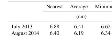
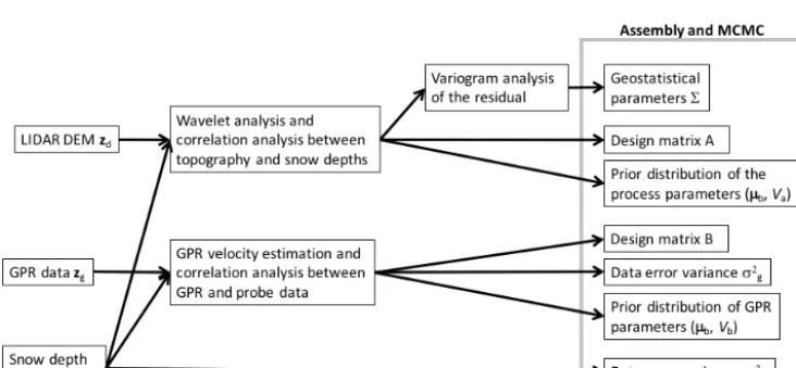
Figure 1. (a)Location of Barrow, Alaska, USA, and Barrow Environmental Observatory (BEO) from Hubbard et al. (2013).(b)NGEE Arctic site with the digital elevation map from the airborne lidar (in meters). The black boxes are the intensive sampling plots (plots A, B, C and D). The white rectangles are the fine-grid snow depth measurements by a snow depth probe. The three black lines represent the 500 m transects.
then develop a Bayesian geostatistical approach to integrate the multiscale datasets to estimate snow depth over the lidar domain. The snow measurement and estimation results are presented in Sect. 4 and discussed in Sect. 5.
2 Data and site descriptions 2.1 Study site
Snow survey data were collected within a study site (approx-imately 750 m×700 m) located on the Barrow Environmen-tal Observatory near Barrow, Alaska, as part of the Depart-ment of Energy’s Next-Generation Ecosystem ExperiDepart-ment (NGEE) Arctic project (Fig. 1). This study domain has been characterized intensively in the NGEE Arctic project, lead-ing to various ecosystem and subsurface datasets, includlead-ing snow depth measurements (Wainwright et al., 2015; Dafflon et al., 2016). Mean annual air temperature at the Barrow site is−11.3◦C and mean annual precipitation is 173 mm (Lil-jedahl et al., 2011). Snowmelt usually ends in early to mid-June. The wind direction is predominantly from east to west throughout the year.
Ice-wedge polygons are prevalent in the region, including low-centered polygons in drained thaw lake basins and high-centered polygons with well-developed troughs in the upland tundra (Hinkel et al., 2003; Wainwright et al., 2015). The dominant plants are mosses (Dicranum elongatum, Sphag-num), lichens and vascular plants (such asCarex aquatilis); plant distribution at the site is governed by surface mois-ture variability (e.g., Hinkel et al., 2003; Zona et al., 2011). There are currently no tall shrubs or woody plants established within the study site, and therefore complex topography is most likely to control the snow depth distribution within the study domain (Sturm et al., 2005; Dvornikov et al., 2015).
Three long transects and four representative plots were chosen within the study site to explore snow variability
and its relationship to topography (Fig. 1). Typical for low-gradient tundra terrain, ice-wedge polygons and microtopo-graphic variations are superimposed on macrotopomicrotopo-graphic trends at the study site. The elevation is higher in the cen-ter of the domain (incen-terstitial upland tundra) and lower near the drainage features in the south. The elevation is also rel-atively lower in the drained thaw lake basins (DTLB) re-gion, which is located in the northeastern and northwest-ern edges of the study site. The four intensive plots (A–D), each 160 m×160 m, were chosen to represent specific poly-gon types or macrotopographic positions within the study area. The three parallel transects, each ∼500m long, were designed to traverse multiple polygon types in a continuous fashion (Hubbard et al., 2013; Wainwright et al., 2015). We refer to those transects by “the 500 m transects”.
2.2 Datasets
Airborne lidar data were collected at the site on 4 Octo-ber 2005 and used to provide a high-resolution DEM of the snow-free ground at 0.5 m×0.5 m resolution (Hubbard et al., 2013). The DEM effectively resolves both micro-and macrotopography at the study site (Fig. 1). The origi-nal reported accuracy is 0.3 m in the horizontal direction and 0.15 m in the vertical direction. To further evaluate the accu-racy of the airborne DEM, we measured the ground surface elevation in September 2011 at 1286 points around the 500 m transects, using a high-precision centimeter-grade RTK dif-ferential GPS (DGPS) system (the reported precision about 2 cm in the horizontal direction and 3 cm in the vertical direc-tion). The root mean square error (RMSE) of the lidar DEM compared to the DGPS data was 6.08 cm.
measure-ments using a snow depth probe were collected. The “fine-grid” dataset was aimed to characterize the fine-scale het-erogeneity by ∼7200 snow depth point measurements (ev-ery ∼0.3 m along transects with a 4 m spacing) across a small domain (∼50 m×50 m) within plots A–D (Liljedahl et al., 2014). This was done using a GPS snow depth probe (Magnaprobe by Snow-Hydro) which had a reported ver-tical precision of <0.01 m and horizontal precision of 2– 10 m. The corner coordinates within each grid were surveyed with the RTK DGPS, while each snow depth point measure-ment was associated with latitude and longitude positional information recorded by the Magnaprobe’s built-in GPS re-ceiver. All the snow depth point measurements were made along regularly spaced transects. Comparisons between co-ordinates surveyed with both the RTK DGPS and the Mag-naprobe’s built-in GPS confirmed constant biases in the hor-izontal directions, which allowed a constant bias adjustment for all the GPS surveyed snow depth point measurements.
A second “coarse-grid” set of snow depth measurements covered the entire area in plots A–D (∼160 m×160 m) with lower sampling density (Peterson et al., 2015a). The coarse-grid snow data were collected using a tile probe, which had a precision of approximately 0.01 m. Snow depth was mea-sured every 8 m along a measurement tape on the five par-allel transects in the coarse grid, which were spaced 40 m apart. The total number of data points was 380 (95 points in each plot). Along the 500 m transects, we used the tile probe along with a measurement tape and measured eight points along each of the three lines. The start and end coordinates of each transect were surveyed with a RTK DGPS and used to georeference the measurement locations.
Ground-based GPR data were acquired over the four study plots and along the three 500 m transects (Peterson et al., 2015b). The instrument (Mala ProEx with 500 MHz an-tenna) was pulled on a sled. In each plot, we acquired the GPR data at 0.1 m intervals (triggered by an odometer wheel) along 37 lines of 4 m spacing. The start and end coordinates of each transect were surveyed with a RTK DGPS and used to georeference the measurement locations. We compared the distance from the wheel with the distance on tape and confirmed that the difference is generally very small at this site. The error of horizontal positioning is estimated to be about 0.1 m. Several of the GPR lines were co-located with the “coarse-grid” snow depth probe measurements. The GPR technique allowed for denser sampling within the plot rela-tive to the snow depth probe, with more than 50 000 points in each plot. Due to the microtopography at this site, the po-sitioning errors between in situ measurements and GPR data could lead to an error in the radar velocity and snow depth estimation. We evaluate the effect of such positioning errors extensively, as described in Sect. 3.1.
The GPR reflection signal from the bottom of snowpack (i.e., the ground surface) was clear, which allowed us to mea-sure the travel time between the top and bottom of snowpack. The GPR processing routine consisted of (1) zero-time
ad-justment, (2) average tracer removal, (3) picking the travel time (manually with automated snapping in the ProMAX® software) of the reflected GPR signal that traveled from the snow surface to the snow-ground interface and back to the snow surface and (4) dividing this travel time by two to ob-tain a one-way travel time between the snow surface and ground surface. We processed the GPR data including travel-time picking before accounting for topography. More details on GPR processing and theory can be found in Annan (2005) and Jol (2009), while more detailed explanation on the use of GPR in the tundra can be found in Hubbard et al. (2013). Differing from previous studies (e.g., Harper and Bradford, 2003), we did not observe echoes from snow layering. This is possibly because of the low antenna frequency (500 MHz), relatively thin snow layers (if present), and the low contrast between various snow layers. In addition, hoar layers or ice layers were not visible in our data or sensed using the probe. Although ice may form at the ground surface, causing the un-certainty of a few centimeters, we did not consider this effect in this study.
Additional campaigns were carried out in 2013–2015 along the 500 m transects only. UAS-based phodar data were collected in July 2013 and 2014 to estimate snow-free ground surface elevation and in May 2015 for estimating snow depth along the transects (Dafflon et al., 2015). To make these measurements, we lifted a consumer-grade digital cam-era (Sony Nex-5R) to about 40 m above ground level us-ing a kite and acquired downward-lookus-ing red–green–blue landscape images, as well as collected some surface ele-vation data (method described in Smith et al., 2009). The reconstruction procedure was performed using a commer-cial computer vision software package (PhotoScan from Ag-isoft LLC). Reconstruction involved automatic image fea-ture detection/matching, strucfea-ture-from-motion and multi-view stereo techniques for 3-D point-cloud generation, and georeferenced mosaic reconstruction (Nolan et al., 2015). High-accuracy georeferencing was enabled by using a net-work of ground control points placed on the ground (in sum-mer) and on the snow (in winter) that were surveyed with a high-precision centimeter-grade RTK DGPS system. The re-constructed phodar surface elevation models at this site show a resolution of 4 cm×4 cm. We investigated the accuracy in detail as described in Sect. 3.2.
3 Methodology
3.1 GPR snow depth analysis
Snow depth can be inferred by multiplying GPR one-way travel time by radar velocity. The radar velocity is deter-mined with the dielectric constant, which depends on snow density in dry snow (Tiuri, et al., 1984; Harper and Brad-ford, 2003). Depending on site conditions, the snow density can vary in both vertical and horizontal directions (Proksch et al., 2015). In this study, we assume that the depth-averaged radar velocity – which is a function of depth-averaged snow density – is sufficient for estimating snow depth. Thus, we compute the radar velocity based on the known snow depth from co-located snow depth probe measurements as (radar velocity)=(probe-based snow depth)/(GPR one-way travel time). In addition, we investigate whether the lateral varia-tions in snow density are significant at our site.
Identifying co-located points between the GPR and snow depth probe measurements, however, is not a trivial task in polygonal ground, since the topography and snow depth can vary significantly within a meter. To address these issues, we investigate the correlations between the radar velocity and the submeter-scale variability of topography. To link the DEM elevation data to the snow depth probe and GPR data, we selected the DEM elevation (0.5 m×0.5 m resolution) and GPR measurement at the nearest locations to the tile probe measurements. We assume that the effect of positioning er-rors is larger near the edge of polygons or in the region where the submeter-scale topographic variability is high. We con-sider that the uncertainty of radar velocity can be reduced by not using the co-located snow depth probe measurements in regions of high submeter-scale variability. To define the submeter-scale variability, we compute the elevation differ-ence within a 1 m radius of each snow depth probe mea-surement. In addition, the reflections from the troughs could originate from the edge of polygons rather than the location right below the GPR instrument. Such an “edge reflection” effect can lead to overestimation of the radar velocity. We as-sume that we could detect the presence of the edge reflection by evaluating the systematic bias (i.e., overestimation) in the radar velocity in relation to the submeter-scale topographic variability.
3.2 UAS-based phodar snow depth analysis
We first evaluate the accuracy of the phodar-derived digital surface model (DSM) by comparing it to the RTK GPS el-evation measurements along the 500 m transects acquired in 2011. Since the phodar-derived DSM was obtained at very high lateral resolution (4 cm×4 cm), it was more prone to noise or small-scale variability (Nolan et al., 2015). As such, we test three schemes to explore the vertical agreement be-tween the two datasets: (1) nearest points, (2) average ele-vation within the 0.5 m radius and (3) minimum eleele-vation
within the 0.5 m radius. We use the same scheme (the best scheme among the three) for determining the snow-free and snow surface elevation at the co-located points. We then com-pare the snow depth estimates from phodar and snow depth probe measurements at co-located points (the May 2015 snow data). Since we assume that the phodar snow depth es-timates would suffer from the same positioning errors asso-ciated with the snow depth probe data as GPR, we eliminate the snow depth probe measurements in the regions where the submeter-scale topographic variability is high.
3.3 Spatial variability analysis of topography and snow depth
To quantify the topographic effects in a complex terrain of ice-wedge polygons and to partition micro- and macrotopog-raphy, we apply the wavelet transform method to the air-borne lidar DEM, which is commonly used for 2-D image processing. The wavelet approach has been applied to DEM in geomorphic studies, including terrain analysis and land-slide analysis (Bjørke and Nilsen, 2003; Kalbermatten, 2010; Kalbermatten et al., 2012). In this transform, a high-pass fil-ter (a mother wavelet) and a low-pass filfil-ter (a father wavelet) are applied to decompose the DEM into four images at each scale: low-pass, high-pass horizontal, high-pass vertical and high-pass diagonal images. The scale is a parameter in the wavelet transform, representing the width of the filter and the scale of topographic variability (Kalbermatten et al., 2012). Depending on the scale of the wavelet transform, the method yields different images, corresponding to different scales of topographic features. We define this wavelet scale as a to-pography separation scale. We consider the low-pass image as macrotopographic elevation (i.e., the smoothed version of the original DEM) and the high-pass diagonal image as microtopographic elevation(i.e., the topographic variability associated with ice-wedge polygon development). Remov-ing the large-scale topography has been done in the previous studies in order to capture or quantify the effect of microto-pography on carbon fluxes (Wainwright et al., 2015) or soil properties (Gillin et al., 2015).
predominant wind direction. With this calculation, the wind factor is smallest in the slope against the wind direction and largest in the slope in line with the wind, which is reasonable and also consistent with visual observations at the site. When the correlation is statistically significant, the metrics are in-cluded in a regression analysis (Davison, 2003) to represent the snow depth as a function of the topographic metrics.
A geostatistical approach has been used to investigate the spatial variability of snow depth as well as the scales of variability (Anderson et al., 2014). The standard geostatisti-cal analysis starts with creating an empirigeostatisti-cal variogram, fol-lowed by estimating the spatial correlation parameters (Dig-gle and Ribeiro Jr., 2007). The spatial correlation parameters include (1) magnitude of variability (or spatial heterogeneity) as variance, (2) fraction of correlated and uncorrelated vari-ability (nugget ratio), (3) spatial correlation length (range) and (4) covariance model (i.e., the shape of decay in the spa-tial correlation as a function of distance), such as exponenspa-tial and spherical models. The covariance models (equivalent to variogram models) can be selected to minimize the weighted sum of squares during variogram fitting.
Such spatial variability and correlation are particularly im-portant for interpolating the sparse in situ snow depth mea-surements. The interpolation can be applied not only for snow depth itself but also for snow surface (snow depth plus elevation) or residual snow depth after removing topographic correlations in the regression analysis. The same geostatis-tical analysis method is therefore performed for snow sur-face and residual snow depth. We used the geoR package in statistical software R (Ribeiro Jr. and Diggle, 2001; https: //www.r-project.org/).
3.4 Bayesian geostatistical estimation method
We first define that the snow depth at each pixel yi (i= 1, . . ., n) is a hidden variable which can be observed only with an added measurement error. In this study, we set the pixel size to 0.5 m×0.5 m, which corresponded to the lidar DEM resolution. The snow depth distribution (or field) is de-fined by a vector y= {yi|i=1, . . ., n}. We integrate three datasets: snow depth probe data zp, GPR data zg and lidar DEMzd. The goal of the estimation is to determine the pos-terior distribution of snow depth conditioned on all the given datasets,p(y|zp,zg,zd). Following a Bayesian hierarchical approach, we divide this posterior distribution into three sets of statistical submodels (Wikle et al., 2001; Wainwright et al., 2014, 2016). First,data modelsrepresent each data value as a function of snow depth at each pixel, depending on dif-ferent data types. Second,process modelsdescribe the spatial distribution of snow depth (i.e., snow depth field) as func-tion of topography and correlafunc-tion parameters. Finally,prior models define the prior information of parameters. The hi-erarchical approach breaks down a complex posterior dis-tribution into a series of simple models and hence enables us to capture complex relationships easily. In addition to the
snow field vector and data vectors, two parameter vectors are defined: the process-model parameter vectora to represent the heterogeneous pattern of snow depth and the data-model parameter vectorbto describe the correlations between the snow depth and the GPR travel time.
We assume a linear model to describe the snow depth field,
y=Aa+τ, (1)
whereAis the design matrix as a function of the topographic metrics as explanatory variables (and hence a function of DEMzd). The process-model parameter vectoradescribes the correlation between the topographic metrics and the snow depth field. We assume that the residual of this correlation τ represents the unexplained variability by the topographic metrics and thatτ is spatially correlated. The residual term τ is described by a multivariate normal distribution with a covariance6, which is determined by a geostatistical anal-ysis (Diggle and Ribeiro Jr., 2007). Although we may in-clude the uncertainty of those geostatistical parameters in the Bayesian estimation (Diggle and Ribeiro Jr., 2007; Lavigne et al., 2017), we assume that those parameters are fixed dur-ing the Bayesian estimation process in this study. This is be-cause we have a large amount of point measurements (snow depth probe data), and also it is known that indirect infor-mation (such as geophysics) does not significantly improve the estimation of geostatistical parameters (Day-Lewis and Lane Jr., 2004; Murakami et al., 2010).
The data model for the snow depth probe measurements defines the snow depth probe datazpas a function of snow depthy:
zp=y+εp. (2)
We assume that the vectorεp is an uncorrelated normally distributed measurement error at each data location with the standard deviation (SD) ofσp. We determine the error based on the precision estimate of each snow depth probe. The snow depth probe data vectorzpfollows a multivariate nor-mal distribution with the mean vectory and the covariance matrixDp, which is a diagonal matrix with diagonal elements ofσp2. Although it is not considered this study, we could in-clude a systematic bias of snow probe measurements as an added shift (Berezovskaya and Kane, 2007).
The data model for the GPR data describes the GPR data zgas a function of the snow depthy at the GPR locations. The GPR data model can be represented by a linear model:
zg=b0+By+εg, (3)
whereBis a matrix, the diagonal elements of which isb1. The error vectorεgis an uncorrelated normally distributed measurement error with the SD ofσg. The SD is computed from comparing the GPR-based snow depth to the probe-based one. At the same time, the GPR data model can be written as a function of the parameter vectorbsuch that
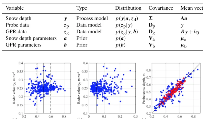
Table 1.Multivariate normal distribution defined for each variable.
Variable Type Distribution Covariance Mean vector
Snow depth y Process model p(y|a,zd) 6 Aa Probe data zp Data model p(zp|y) Dp y GPR data zg Data model p(zg|y,b) Dg By+b0 Snow depth parameters a Prior p(a) Va µa
GPR parameters b Prior p(b) Vb µb
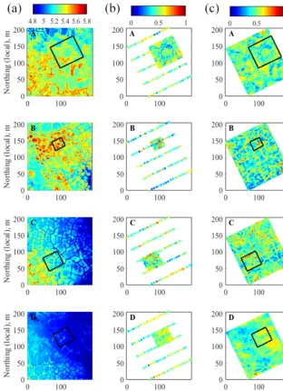
Figure 2.Radar velocity as a function of(a)co-located snow depth measured by a snow depth probe and(b) elevation difference (i.e., topographic variability) within 1 m.(c)Comparison between the probe-derived and GPR-derived snow depth at all the co-located locations (blue circles) and at selected locations (red circles) where topographic variability is low. In(a), the black vertical line is the median snow depth, and the dotted lines are±1 SD from the median snow depth. In(b), the black line is the cutoff elevation difference of 0.05 m.
whereYis the design matrix with the first column beingy, and the second column being all one. The parameter vec-torb= {b1, b0}represents the linear correlations between the GPR data and snow depth. This alternative model is useful during the estimation procedure described below. The GPR data vectorzgfollows a multivariate normal distribution with the mean vectoryand the covariance matrixDgthat is a di-agonal matrix with didi-agonal elements ofσg2.
The posterior distribution of the snow depth conditioned on the datasets p(y|zd,zp,zg)is a marginal distribution of p(y,a,b|zd,zp,zg). By applying Bayes’ rule and following the conditional dependencies defined above, we can decom-pose this posterior distribution as
p y,a,b|zd,zp,zg
∝p zg|y,bp zp|yp (y|a,zd) p(a)p(b). (5)
Table 1 defines all the distributions on the right-hand side of Eq. (5) based on the models defined in Eqs. (1)–(4). We also assume multivariate normal distributions for the prior distributions of the parameter vectorsaandb. The posterior distribution in Eq. (5) can be computed using the Markov-chain Monte Carlo (MCMC) method (Gamerman and Lopes, 2006). Since all the distributions are defined as multivariate normal distributions, it is possible to use efficient Gibbs’ al-gorithm. The MCMC procedure is described in Appendix A. The convergence can be confirmed by the Geweke conver-gence diagnostic (Geweke, 1992). The entire workflow is in-cluded in Appendix B.
4 Results
4.1 Snow depth measurements 4.1.1 GPR radar velocity analysis
Our results (based on the GPR data and tile probe data col-lected in May 2012) indicate that the estimated radar veloc-ity itself does not have a systematic dependency on (or trend with) the snow depth or submeter-scale variability of topog-raphy in May 2012 (Fig. 2a and b). The correlation coeffi-cient between the radar velocity and snow depth is 0.11 and between the radar velocity and submeter-scale variability is 0.15. The variability of the radar velocity, however, depends on those two factors (i.e., the variability of snow depth and topography). Hence, the variability is higher in areas with shallower snow depths (Fig. 2a). The SD of the radar veloc-ity is 0.039 m ns−1at the snow depth smaller than 1 SD mi-nus the median snow depth and is 0.019 m ns−1at snow depth larger than 1 SD plus the median. The radar velocity variabil-ity is higher also in localized regions of large submeter-scale topographic variability (Fig. 2b). The SD of the radar veloc-ity is 0.015 m ns−1 at the submeter-scale topographic vari-ability (i.e., elevation difference within a 1 m radius) smaller than 0.05 m, and 0.036 m ns−1at the one larger than 0.05 m. By selecting the points with the submeter-scale topographic variability<0.05 m, we obtained a mean radar velocity of 0.25 m ns−1, which was used for subsequent analysis.
Figure 3.Elevation and snow depth in plots A, B, C and D. Panel(a)is lidar DEM (in meters), panel(b)is the probe measured snow depth (in meters), and panel(c)is the interpolated snow depth estimated using GPR (in meters).
the snow depth probe measurements (Fig. 2c). The correla-tion between the measured and estimated snow depth is high (the correlation coefficient is 0.88), with the RMSE being 5.4 cm and no significant under- or overestimation (the mean bias error −0.16 cm). The selected points in the regions of low submeter-scale topographic variability (red circles) are more tightly distributed around the one-to-one line. In these regions, the RMSE of GPR-based snow depth improved to 2.9 cm with a increased correlation coefficient between the GPR-based and probe-based snow depth to 0.94. These re-sults confirm that snow density variations are limited, and using a constant mean GPR velocity is acceptable.
4.1.2 Snow depth measurements in different polygon types
macrotopo-graphic trends. Plot C is gradually sloping down towards the east, and plot D has a depression (i.e., DTLB) in the north-eastern half.
In Fig. 3b shows the snow depth probe data collected us-ing the fine-grid and coarse-grid scheme collected in May 2012. The fine-grid data reveal the detailed heterogeneity of snow depth around a single polygon. For example, the fine-grid data in plot A show the snow depth distribution in a low-centered polygon, including thin snow along the polygon rim and thick snow at the polygon center and trough. Comparison of the fine-grid snow data with the DEM reveals the microto-pographic effect such that the troughs and center of the poly-gon have larger snow depth. The coarse-grid dataset covers the entire plot, although it is much more difficult to ascertain the relationship between the snow depth and microtopogra-phy. The snow depth probe data show that the snow depth is highly variable, ranging from 0.2 to 0.8 m in a single plot.
In Fig. 3c, the May 2012 snow depth was estimated from GPR using a fixed radar velocity 0.25 m ns−1along the lines within the plots, and then interpolated with a simple linear interpolation in between the lines. The high-resolution GPR snow depth estimates are useful for determining if micro-topographic features can influence the distribution of snow depths across each study plot. The high-resolution snow es-timates over the large area allow us to visually identify the macrotopographic control on snow depth. In plot C, for ex-ample, the snow depth does not have an increasing or de-creasing trend, even though the elevation gradually decreases towards east. Plot D, in contrast, has more snow accumula-tion in the eastern part of the domain, which is in the depres-sion associated with DTLB.
4.1.3 Phodar-based snow depth measurements
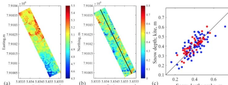
In the region of the 500 m transects, the phodar-derived snow-free DSMs (Fig. 4a) collected in July 2013 and August 2014 were first compared with the RTK DGPS data (acquired in 2011) in Table 2, using the different schemes to identify co-location. We included the results of both years to confirm the consistency between the two snow-free DSM products at the same terrain. Although all the schemes yielded an excel-lent accuracy (the RMSE less than 7.0 cm), taking the aver-age provides the lowest RMSE in both years (6.41 cm in 2013 and 6.19 cm in 2014), which is approximately the same as the lidar data (RMSE=6.08 cm). The phodar-derived snow depth estimates in May 2015 were obtained by differencing the snow surface and snow-free DSM (Fig. 4b). The com-parison between the phodar-based snow estimates and the snow depth probe data is favorable (Fig. 4c), with a RMSE of 6.0 cm. When we removed the points that had a large submeter-scale topographic variability in the vicinity (in the same way and the same cutoff values as the GPR snow depth analysis), the RMSE improved to 4.6 cm (Fig. 4c).
The phodar-derived snow depth (Fig. 4b) around the 500 m transects in May 2015 reveals a similar pattern of snow
dis-Table 2. Root mean square error (RMSE) between the phodar-derived DSM and RTK DGPS elevation measurements based on the three schemes: nearest neighbor, average, and minimum eleva-tion within the 0.5 m radius.
Nearest Average Minimum
(cm)
July 2013 6.88 6.41 6.62 August 2014 6.40 6.19 6.34
tribution as the GPR data in Fig. 3, having deeper snow in the troughs and the centers of low-centered polygons. The high-resolution image of the phodar data reveals more detail of the microtopographic effect than the interpolated image of the GPR data, particularly in the narrow troughs. The large aerial coverage also shows the minimal effect of macroto-pography: while the elevation decreases towards south, the snow depth does not have a large-scale trend.
4.2 Snow depth variability over tundra
4.2.1 Variability among different polygon types Figure 5 shows the box plots of the snow depth, elevation and microtopographic elevation (1 elevation) in each plot measured in May 2012. We used the coarse-grid snow depth probe measurements, since the samples are uniformly dis-tributed over each plot. The median snow depth (Fig. 5a) is fairly similar among four plots, even though they have dif-ferent geomorphologic features and polygon types. Tukey’s pairwise comparison test (Table 3) shows that only plot B (small high-centered polygons) is significantly different from the other plots.
Figure 4. (a) Phodar-derived DSM in meters (August 2014),(b)phodar-derived snow depth in meters (May 2015) and(c)comparison between the phodar-based and probe-based snow depth at all the locations (blue circles) and at selected locations (red circles) having low topographic variability (the sub-meter elevation variability less than 0.05 m). The black line in(b)represents the snow depth probe measurements every 3 m along the 500 m transect.
Figure 5.Box plots of(a)snow depth,(b)elevation and(c) micro-topographic elevation in plots A–D.
Table 3.pvalues from Tukey’s pairwise comparison test for each pair of the plots.
Plots Snow depth
A–B 6.34×10⁻³ A–C 0.982 A–D 0.998 B–C 1.72×10⁻³ B–D 3.55×10⁻³ C–D 0.997
4.2.2 Correlations between snow depth and topographic indices in May 2012
Among the topographic indices of macro- and microtopog-raphy, the snow depth in May 2012 (measured by the snow depth probe) was significantly correlated only to the micro-topographic elevation for all plots (Fig. 6a). The correlation coefficient changes with the scale of the wavelet transform that separates micro- and macrotopography. The correlation coefficient is up to−0.8 at plot B (small high-centered poly-gons) and up to −0.7 at all the data points. The correla-tion coefficient is different among different plots (i.e.,
dif-Figure 6.Correlation coefficients between snow depth and topo-graphic metrics as a function of the wavelet scale:(a)the micro-topographic elevation and(b)the wind factor of macrotopography. The different colors represent different plots (plots A–D) or all the data (All). Each dash line represents the scale that maximize the magnitude of the correlation coefficient.
ferent polygon types); the correlation is less significant at plot D (low-centered polygons in DTLB) than other plots. The best correlation (i.e., the largest absolute value) can be achieved at a different scale in each plot (plot B<plot A and plot C<plot D).
reported (the elevation difference in their domain was more than 60 m).
4.2.3 Geostatistical analysis of snow depth
Spatial correlation exists for all three variables in May 2012: snow depth, snow surface and residual snow depth after re-moving the correlation to the microtopographic elevation (Table 4). The correlation range is less than 20 m for the snow depth, which is consistent with the large variability in a short distance. The snow surface, in contrast, has a larger correlation range (253 m). The estimation of a snow surface height (elevation+snow depth) effectively removes the in-fluence of microtopography, resulting in much a larger cor-relation range. The variance is comparable between the snow depth and snow surface, while the variance is much lower in the residual snow depth, since the topographic correlation explains a large portion of the snow depth variability.
4.3 Snow depth estimation based on lidar DEM Based on the snow-topography analysis in Sect. 4.2, we in-cluded the linear correlation between snow and microtopo-graphic elevation in Eq. (1) to describe the snow variability in May 2012. We used the Shapiro–Wilk normality test to confirm that the residual of the linear correlation, defined by τ in Eq. (1), follows a normal distribution (thep value of rejecting this hypothesis was 0.21). The first column of the design matrixAis the microtopographic elevation at all the pixels, and the second one is a vector of all 1s. The parameter vectorais a 2-by-1 vector with the linear correlation param-eters (slope and intercept). The Bayesian method (Sect. 3.4) yielded 10 000 equally likely fields of the snow depth from the posterior distribution in Eq. (5).
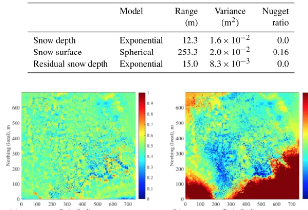
The Bayesian estimated mean snow depth field over the full study domain in May 2012 (Fig. 7a) captures the ef-fects of microtopography, such as more snow accumulation in polygon troughs and centers of low-centered polygons. The snow depth does not have any large-scale trends over the full study domain, which is different from the lidar DEM in Fig. 1b, but consistent with the interpolated GPR snow depths depicted in Fig. 3c and the measured UAS snow depth measurements depicted in Fig. 4b. The variability is larger in the southern region where there are high-centered polygons with deep troughs.
In addition, we compared this result (Fig. 7a) with the mean field from estimating the snow surface elevation and subtracting the ground surface elevation (Fig. 7b). In this es-timation, we used the same Bayesian algorithm described in Sect. 3.4, except that we removed the topographic correla-tions and assumed a standard geostatistical model for snow surface (Diggle and Ribeiro Jr., 2007). In other words, we had the same algorithm except that we modified Eq. (1) to y=c−z+τ, where y+zrepresents the surface elevation andcis a constant. Although the two mean fields (Fig. 7) are
similar in the central regions that have many measurements, the regions without any measurements have a significant de-viation. This is because the snow surface estimation did not capture the change in macrotopography (e.g., the drainage feature in the southern part of the domain).
The estimated SD of the Bayesian-derived snow depth over the study domain (Fig. 8a) also shows a significant dif-ference from the one based on the snow surface interpolation (Fig. 8b). This SD represents the uncertainty in the estima-tion. In both cases, the SD is smaller near the measurement locations along the transects and within the four plots. How-ever, when the topographic correlation is included (Fig. 8a), the SD increases more rapidly as the pixel is farther away from the data points. This is due to the fact that the spatial correlation range is small for the residual snow depth after removing the topographic correlation (Table 4).
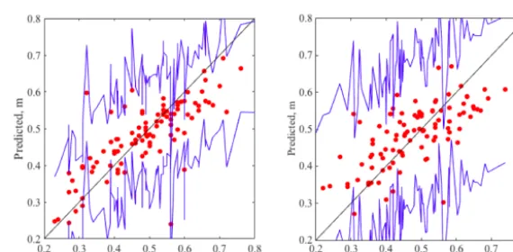
Validation of the snow depth estimates over the study area (plots A–D and the 500 m transects) was performed by com-paring the estimates with the snow depth probe data (May 2012) not used in the Bayesian snow depth estimation. We selected 100 points randomly from the snow depth probe data (all the locations in plots A–D and the 500 m tran-sects), using a uniform distribution. The validation results (Fig. 9) show that the estimated confidence interval captures the probe-measured snow depth. The estimated snow depth is distributed along with the one-to-one line without any sig-nificant bias. The estimation, including the topographic cor-relation (Fig. 9a), has a tighter confidence interval and better estimation results than the one from interpolating the snow surface (Fig. 9b). The RMSE for the Bayesian method of es-timating snow depth including the topographic correlation is 6.0 cm, while the RMSE for the interpolated snow surface is 8.8 cm.
5 Discussion
5.1 Different observational platforms
vicin-Table 4.Estimated geostatistical parameters and covariance models for snow depth, snow surface and residual snow depth.
Model Range Variance Nugget (m) (m2) ratio
Snow depth Exponential 12.3 1.6×10⁻² 0.0 Snow surface Spherical 253.3 2.0×10⁻² 0.16 Residual snow depth Exponential 15.0 8.3×10⁻³ 0.0
Figure 7.The estimated mean snow depth across the site (in meters) based on(a)the proposed Bayesian method including the correlation to microtopography and(b)the kriging-based interpolation of the snow surface. The spatial extent is the same as Fig. 1b.
ity of the calibration points, suggesting the impact of posi-tioning errors. Third, there was no systematic trend in the radar velocity as a function of the snow depth or topographic positions. We developed a simple methodology (described in Sect. 3.1) to select co-located calibration points based on the submeter-scale variability of topography, which proved to be useful to compute accurate velocity. We note that – even though the depth-averaged radar velocity and hence the depth-averaged snow density have little variability over the space – the snow density could be variable vertically along the depth. From snow coring, we indeed found some layers of ice created by winter rain events that were not detected by the GPR or with probe; it is possible that there might be a difference in the depth-averaged density and radar velocity at a later time, when the snow pack starts to melt in a hetero-geneous manner.
UAS-based phodar provided an attractive alternative for estimating snow depth at high resolution over a large area. With much less labor and time, UAS-based phodar can pro-vide many more sample points than GPR. The phodar-based snow depth, however, was less accurate than ground-based GPR or snow depth probe measurements (RMSE=6.0 cm). The main contribution of this error resulted from the snow-free elevation, since RMSE for the surface DSM is around 6 cm. We note that the RMSE of 6.0 cm is still significantly more accurate than the previous lidar and other airborne sur-veys (e.g., Deems et al., 2013; Harpold et al. 2014; Nolan et al., 2015).
The phodar-based approach is expected to continue its tra-jectory of continuous improvements in terms of technical
as-pects, ease of use and accuracy. At the time of our campaign, we were allowed to use only a kite due to regulations, which led to a limited number of pictures that could be used to re-construct the DSM. The accuracy will significantly improve with the use of a light unmanned aerial vehicle (UAV). Al-though UAS-based lidar acquisition technology continues to improve (e.g., Anderson and Gaston, 2013), as is expected to be a powerful alternative to characterize snow, the lidar de-vice is still significantly more expensive than a conventional camera (roughly by factor of 100). Given that the vegetation height is fairly small in the Arctic tundra, the phodar tech-nique is an affordable alternative.
Figure 8.The estimated standard deviation of snow depth across the site (in meters) based on(a)the proposed Bayesian method, including the correlation to microtopography, and(b)the kriging-based interpolation of the snow surface. The spatial extent is the same as Fig. 1b.
Figure 9.Estimated mean and confidence intervals from the Bayesian method, compared to the probe-measured snow depth by(a)using the correlation to microtopography and(b)interpolating the snow surface. The red circles represent the snow depth at the validation locations (the snow depth probe measurements not used in the estimation), the blue lines are the confidence intervals based on the standard deviation (SD) multiplied by 1.9 (94 % confidence intervals), and the black lines are the one-to-one line.
5.2 Snow depth variability
The end-of-year snow depth distribution at the ice-wedge polygons was highly variable over a short distance in May 2012. The snow depth was, however, significantly corre-lated with the microtopographic elevation, suggesting that the snow depth could be described by microtopography. The wind-blown snow transport leads to significant snow redis-tribution and fills microtopographic lows (i.e., troughs and centers of low-centered polygons) with thicker snow pack (e.g., Pomeroy et al., 1993). The redistribution also results in the smooth snow surface, following the macrotopogra-phy. The exception was observed at the edge of the DTLB, where the abrupt change in macrotopography led to increased accumulation in the depression. This is a similar effect to that observed along the riverbanks by Benson and Sturm (1993). Although the tundra ecosystem studies have focused on the effect of microtopography (e.g., Zona et al., 2011), the macrotopography also may be important when we character-ize snow distribution over a larger area.
The “average” (or median) snow depth over a hundred-meter scale (i.e., the size of plots A–D), however, was fairly
uniform across the site despite the different polygon types in May 2012. Plots A (well-defined low-centered polygons) and C (flat-centered polygons), for example, have different poly-gon types, but they have a similar median snow depth. This is because microtopography and microtopographic features (i.e., polygon troughs, rims) mainly control the snow distri-bution. Plot B (small high-centered polygons) is an excep-tion, having smaller median snow depth than the other plots. Plot B has the largest variability in microtopography, charac-terized by the small round high-centered polygons, like nu-merous small mounds (Fig. 3). Such mounds are prone to erosion by the wind, and hence lead to less snow trapping and accumulation.
present site, where different types and sizes of polygons mix together. Although we used the same scale for the estimation, an improved polygon delineation algorithm will possibly en-able us to separate micro- and macrotopography in the future (e.g., Wainwright et al., 2015).
5.3 Snow depth estimation
The developed Bayesian approach enabled us to estimate the snow depth distribution over a large area based on the lidar DEM and the correlation between the snow depth and to-pography. Although this paper only used the ground-based GPR and snow depth probe measurements collected at the same time, phodar could be easily included in the same framework. The Bayesian method allowed us to integrate three types of datasets (lidar DEM, snow depth probe and GPR) in a consistent manner and also provided the uncer-tainty estimate for the estimated snow depth. Taking into account the topographic correlation explicitly improved the accuracy of estimation significantly (RMSE=6.0 cm), com-pared to interpolating the snow surface and subtracting the DEM (RMSE=8.8 cm).
Our approach can be extended to snow estimates over both time and space. The correlations between snow depth and to-pography may change over time. In early and later winter, for example, the snow depth would be more affected by cur-vature and slope of microtopography, since the microtopo-graphic lows (troughs and centers of the low-centered poly-gons) are not filled by snow. It would be possible to quan-tify the seasonal changes in the topography–snow correla-tions by designing a full season ground-based measurement campaign and acquisition of remote sensing snow depth mea-surements (by phodar or lidar) that monitored the same site over several years to account for interannual variability. The Bayesian method presented here is flexible enough to ac-count for changes in parameters over time for the spatiotem-poral data integration (e.g., Wikle et al., 2001). Although physically based snow distribution models can be used for the same purposes (e.g., Pomeroy et al., 1993; Liston and Sturm, 1998, 2002), it is difficult to parameterize all the pro-cesses, such as sublimation and turbulent transport. Our data-driven approach provides a powerful alternative to distribute snow depth based on various datasets.
6 Summary
In this study, we explored various strategies to estimate the end-of-year snow depth distribution over an Arctic ice-wedge polygon tundra region. We first developed an effective methodology to calibrate GPR and phodar in the presence of submeter-scale variability of topography. We then investi-gated the characteristics and accuracy of three observational platforms: snow depth probe, GPR and phodar. The phodar-derived snow depth estimates have great potential for accu-rately characterizing snow depth over larger regions (with an RMSE of 4.6 cm), relative to the in situ snow depth measure-ments. The GPR snow depth estimates were slightly more accurate (with an RMSE of 2.9 cm), but they required con-siderable more effort to obtain and require complex post-processing to minimize errors associated with radar position-ing.
We investigated the spatial variability of the snow depth and its dependency on the topographic metrics. At the peak snow depth during our data acquisition, the snow depth was highly correlated with microtopographic elevation (the corre-lation coefficient of up to−0.8), although it was highly vari-able over short distances (the correlation range of 12.3 m). It is considered that the wind redistribution filled the micro-topography by snow and created a snow surface following macrotopography at the site. The challenge was to separate macro- and microtopography, since the separation scale was not arbitrary and depended on the polygon size. The wavelet analysis provided an effective approach to identify this sepa-ration scale.
The Bayesian method was effective at integrating different measurements to estimate snow depth distribution over the site. Although our estimation is based on the data collected from a one-time campaign, and the correlations to topog-raphy may change over time, the approach developed here is expected to be applicable for estimating both spatial and temporal variability of snow depth at other sites and in other landscapes.
Appendix A: MCMC derivation
In MCMC, we sample each variable sequentially conditioned on all the other variables. In other words, when we update one variable (or one vector), we assume that the other vari-ables are known and fixed. After sampling thousands of sets of the variables, the distribution of those samples converges to the posterior distribution. Each vector is sampled as fol-lows.
The snow depth field is sampled from the distribution p(y|·)=p(y|a,b,zd,zg,zp)
∝ p(zg|y,b) p(zp|y) p(y|a,zd), (A1) where “·” represents all the other variables. The tion is decomposed to a series of small conditional distribu-tions defined in Table 1. Similarly, we can sample the snow-process parameters a and GPR-data parameter b from the distributions
p(a|·)=p(a|y,zd) ∝ p(y|zd,a)p(a), (A2) p(b|·)=p(b|y,zg) ∝ p(zg|y,b)p(b). (A3) Since all the distributions in Eqs. (A1)–(A3) are multivariate Gaussian, we can use the conjugate prior to compute an an-alytical form of each distribution. Each distribution is mul-tivariate Gaussian with the covariance and mean vector de-fined in Table A1. In the Gibbs sampling algorithm, we sam-ple each variable vector sequentially until the distributions are converged.
Appendix B: Bayesian estimation workflow
Table A1.Posterior distributions during the Gibbs sampling.
Variable Covariance,Q Mean vector
Snow depth y (BTD−g1B+Dp−1+6−1)−1 Q
BTD−g1(zg−b0)+D−p1zp+6−1Aa
Snow depth parameters a (AT6−1A+V−a1)−1 Q
AT6−1y+V−a1µa
GPR parameters b (HTD−g1H+V−b1)−1 Q
BTD−g1 zg−b0+V−b1µb
Competing interests. The authors declare that they have no conflict of interest.
Acknowledgements. The Next-Generation Ecosystem Experiments (NGEE) Arctic project is supported by the Office of Biological and Environmental Research in the DOE Office of Science. This NGEE Arctic research is supported through contract number DE-AC0205CH11231 to Lawrence Berkeley National Laboratory. We gratefully acknowledge Stan Wullschleger in Oak Ridge National Laboratory, project PI. We thank Craig Tweedie at University of Texas, El Paso, for providing the lidar dataset and Sergio Vargas from University of Texas, El Paso, for providing kite-based landscape imaging advice. We also thank G. Chambon, N. Eckert and one anonymous reviewer for the helpful comments.
Edited by: G. Chambon
Reviewed by: N. Eckert and one anonymous referee
References
Anderson, B. T., McNamara, J. P., Marshall, H. P., and Flores, A. N.: Insights into the physical processes controlling correlations be-tween snow distribution and terrain properties, Water Resour. Res., 50, 4545–4563, 2014.
Anderson, K. and Gaston, K. J.: Lightweight unmanned aerial vehi-cles will revolutionize spatial ecology, Front. Ecol. Environ., 11, 138–146, 2013.
Annan, A. P.: Ground penetrating radar, in near surface geophysics, in: Investigations in Geophysics, edited by: Butler, D. K., Soci-ety of Exploration Geophysicists, Tulsa, OK, USA, 13, 357–438, 2005.
Benson, C. S. and Sturm, M.: Structure and wind transport of sea-sonal snow on the Arctic slope of Alaska, Ann. Glaciol., 18, 261– 267, 1993.
Berezovskaya, S. and Kane, D. L.: Measuring snow water equiva-lent for hydrological applications: part 1, accuracy of observa-tions, in: 16th International Northern Research Basins Sympo-sium and Workshop Petrozavodsk, Russia, 27 August–2 Septem-ber 2007, available at: http://resources.krc.karelia.ru/krc/doc/ publ2007/SYMPOSIUM_029-35.pdf (last access: 12 March 2017), 2007.
Bowling, L. C., Kane, D. L., Gieck, R. E., Hinzman, L. D., and Lettenmaier, D. P.: The role of surface storage in a low-gradient Arctic watershed, Water Resour. Res., 39, 1087, doi:10.1029/2002WR001466, 2003.
Bjørke, J. T. and Nilsen, S.: Wavelets applied to simplification of digital terrain models, Int. J. Geogr. Inf. Sci., 17, 601–621, 2003. Brown, J.: Tundra soils formed over ice wedges, northern Alaska,
Soil Sci. Soc. Am. J., 31, 686–691, 1967.
Callaghan, T. V., Johansson, M., Brown, R. D., Groisman, P. Y., Labba, N., Radionov, V., Bradley, R. S., Blangy, S., Bulygina, O. N., Christensen, T. R., Colman, J. E., Essery, R. L. H., Forbes, B. C., Forchhammer, M. C., Golubev,V. N., Honrath, R. E., Ju-day, G. P., Meshcherskaya, A. V., Phoenix, G. K., Pomeroy, J., Rautio, A., Robinson, D. A., Schmidt, N. M., Serreze, M. C., Shevchenko, V. P., Shiklomanov, A. I., Shmakin, A. B., Sköld, P., Sturm, M., Woo, M.-k., and Wood, E. F.: Multiple Effects of
Changes in Arctic Snow Cover, AMBIO, 40, Supplement 1, 32– 45, doi:10.1007/s13280-011-0213-x, 2011.
Clein, J. S. and Schimel, J. P.: Microbial activity of tundra and taiga soils at sub-zero temperatures, Soil Biol. Biochem., 27, 1231– 1234, 1995.
Dafflon, B., Hubbard, S., Ulrich, C., and Peterson, J. E.: Low-altitude remote sensing dataset of DEM and RGB mosaic for AB corridor on July 13 2013 and L2 corridor on July 21 2013, doi:10.5440/1177858, 2014.
Dafflon, B., Hubbard, S., Ulrich, C., Peterson, J., Wu, Y., Wainwright, H., and Kneafsey, T. J.: Geophysical estimation of shallow permafrost distribution and properties in an ice-wedge polygon-dominated Arctic tundra region, Geophysics, 81, WA247–WA263, 2016.
Davison, A. C.: Statistical models, in: Cambridge Series in Statisti-cal and Probabilistic Mathematics (No. 11), Cambridge Univer-sity Press, Cambridge, UK, 2003.
Day-Lewis, F. D. and Lane Jr., J. W.: Assessing the resolution-dependent utility of tomograms for geostatistics, Geophys. Res. Lett., 31, L07503, doi:10.1029/2004GL019617, 2004.
Deems, J. S., Painter, T. H., and Finnegan, D. C.: Lidar measure-ment of snow depth: a review, J. Glaciol., 59, 467–479, 2013. Derksen, C., Silis, A., Sturm, M., Holmgren, J., Liston, G.,
Hunting-ton, H., and Solie, D.: Northwest Territories and Nunavut Snow Characteristics from a Subarctic Traverse: Implications for Pas-sive Microwave Remote Sensing, J. Hydrometeorol., 10, 448– 463, doi:10.1175/2008JHM1074.1, 2009.
Diggle, P. and Ribeiro Jr., P. J.: Model-based geostatistics, Springer Science & Business Media, New York, USA, 2007.
Dvornikov, Y., Khomutov, A., Mullanurov, D., Ermokhina, K., Gubarkov, A., and Leibman, M.: GIS and field data based mod-elling of snow water equivalent in shrub tundra, Fennia, 193, 53– 65, doi:10.15356/2076-6734-2015-2-69-80, 2015.
Engstrom, R., Hope, A., Kwon, H., Stow, D., and Zamolodchikov, D.: Spatial distribution of near surface soil moisture and its rela-tionship to microtopography in the Alaskan Arctic coastal plain, Hydrol. Res., 36, 219–234, 2005.
Gamerman, D. and Lopes, H. F.: Markov Chain Monte Carlo – Stochastic simulation for Bayesian inference, 2nd Edn., Chap-man & Hall/CRC, Boca Raton, USA, 2006.
Gamon, J. A., Kershaw, G. P., Williamson, S., and Hik, D. S.: Mi-crotopographic patterns in an arctic baydjarakh field: do fine-grain patterns enforce landscape stability?, Environ. Res. Lett., 7, 015502, doi:10.1088/1748-9326/7/1/015502, 2012.
Geweke, J.: Evaluating the accuracy of sampling-based approaches to calculating posterior moments, in: Bayesian Statistics 4, edited by: Bernado, J. M., Berger, J. O., Dawid, A. P., and Smith, A. F. M., Clarendon Press, Oxford, UK, 1992.
Gillin, C., Bailey, S., McGuire, K., and Gannon, J.: Mapping of Hy-dropedologic Spatial Patterns in a Steep Headwater Catchment, Soil Sci. Soc. Am. J., 79, 440, doi:10.2136/sssaj2014.05.0189, 2015.
Gusmeroli, A. and Grosse, G.: Ground penetrating radar detection of subsnow slush on ice-covered lakes in interior Alaska, The Cryosphere, 6, 1435–1443, doi:10.5194/tc-6-1435-2012, 2012. Gusmeroli, A., Wolken, G., and Arendt, A.: Helicopter-borne radar
Harper, J. T. and Bradford, J. H.: Snow stratigraphy over a uniform depositional surface: spatial variability and measurement tools, Cold Reg. Sci. Technol., 37, 289–298, 2003.
Harpold, A. A., Guo, Q., Molotch, N., Brooks, P. D., Bales, R., Fernandez-Diaz, J. C., Musselman, K. N., Swetnam, T. L., Kirch-ner, P., Meadows, M. W., Flanagan, J., and Lucas, R.: LiDAR-derived snowpack data sets from mixed conifer forests across the Western United States, Water Resour. Res., 50, 2749–2755, doi:10.1002/2013WR013935, 2014.
Hinkel, K. M., Eisner, W. R., Bockheim, J. G., Nelson, F. E., Peter-son, K. M., and Dai, X.: Spatial extent, age, and carbon stocks in drained thaw lake basins on the Barrow Peninsula, Alaska, Arct. Antarct. Alp. Res., 35, 291–300, 2003.
Hirashima, H., Kodama, Y., Sato, N., Ohata, T., Yabuki, H., and Georgiadi, A.: Nonuniform Distribution of Tundra Snow Cover in Eastern Siberia, J. Hydrometeorol., 5, 373–389, doi:10.1175/1525-7541(2004)005<0373:NDOTSC>2.0.CO;2, 2004.
Hubbard, S. and Rubin, Y.: Hydrogeophysics, Chapter 1, in: Hydro-geophysics, editd by: Rubin, Y. and Hubbard, S., Elsevier, Ams-terdam, Netherlands, 2005.
Hubbard, S. S., Gangodagamage, C., Dafflon, B., Wainwright, H., Peterson, J. E., Gusmeroli, A., Ulrich, C., Wu, Y., Wilson, C., Rowland, J., Tweedie, C., and Wullschleger, S. D.: Quantifying and relating land-surface and subsurface variability in permafrost environments using LiDAR and surface geophysical datasets, Hydrogeol. J., 21, 149–169, 2013.
Jansson, J. K. and Ta¸s, N.: The microbial ecology of permafrost, Nat. Rev. Microbiol., 12, 414–425, doi:10.1038/nrmicro3262, 2014.
Jol, H. M.: Ground Penetrating Radar Theory and Applications, El-sevier Science, Amsterdam, Netherlands, 2009.
Kane, D. L., Hinzman, L. D., Benson, C. S., and Liston, G. E.: Snow hydrology of a headwater Arctic basin: 1. Physical mea-surements and process studies, Water Resour. Res., 27, 1099– 1109, doi:10.1029/91WR00262, 1991.
Kalbermatten, M.: Multiscale analysis of high resolution digital el-evation models using the wavelet transform, thesis, Ecole Poly-technique Federale de Lausanne, Lausanne, Switzerland, 2010. Kalbermatten, M., Van De Ville, D., Turberg, P., Tuia, D., and Joost,
S.: Multiscale analysis of geomorphological and geological fea-tures in high resolution digital elevation models using the wavelet transform, Geomorphology, 138, 352–363, 2012.
Lavigne, A., Eckert, N., Bel, L., Deschâtres, M., and Parent, E.: Modelling the spatio-temporal repartition of right-truncated data: an application to avalanche runout altitudes in Hautes-Savoie, Stoch. Env. Res. Risk A., 31, 629–644, doi:10.1007/s00477-016-1301-z, 2017.
Leffingwell, E. de K.: Ground-ice wedges: The dominant form of ground-ice on the north coast of Alaska, J. Geol., 23, 635–654, 2015.
Liljedahl, A. K., Ulrich,U., Wullshelger, S., and Hinzman, L.: Snow Depth and Density at End-of-Winter for NGEE Areas A, B, C and D, Barrow, Alaska, 2012–2014, doi:10.5440/1236472, 2014. Liljedahl, A. K., Hinzman, L. D., Harazono, Y., Zona, D., Tweedie, C. E., Hollister, R. D., Engstrom, R., and Oechel, W. C.: Nonlin-ear controls on evapotranspiration in arctic coastal wetlands, Bio-geosciences, 8, 3375–3389, doi:10.5194/bg-8-3375-2011, 2011.
Liljedahl, A. K., Boike, J., Daanen, R. P., Fedorov, A. N., Frost, G. V., Grosse, G., Hinzman, L. D., Y., Iijma, Jorgenson, J. C., Matveyeva, N., Necsoiu, M., Raynolds, M. K., Romanovsky, V. E., Schulla, J., Tape, K. D., Walker, D. A., Wilson, C. J., Yabuki, H., and Zona, D.: Pan-Arctic ice-wedge degradation in warming permafrost and its influence on tundra hydrology. Nat. Geosci., 9, 312–318, doi:10.1038/ngeo2674, 2016.
Liston, G. E. and Sturm, M.: A snow–transport model for complex terrain, J. Glaciol., 44, 498–516, 1998.
Liston, G. E. and Sturm, M.: Winter precipitation patterns in arctic Alaska determined from a blowing-snow model and snow-depth observations, J. Hydrometeorol., 3, 646–659, 2002.
MacKay, J. R.: Thermally induced movements in ice-wedge poly-gons, western Arctic coast: a long-term study, Geogr. Phys. Quatern., 54, 41–68, 2000.
Machguth, H., Eisen, O., Paul, F., and Hoelzle, M.: Strong spatial variability of snow accumulation observed with helicopter borne GPR on two adjacent Alpine glaciers, Geophys. Res. Lett., 33, L13503, doi:10.1029/2006GL026576, 2006.
Murakami, H., Chen, X., Hahn, M. S., Liu, Y., Rockhold, M. L., Vermeul, V. R., Zachara, J. M., and Rubin, Y.: Bayesian approach for three-dimensional aquifer characterization at the Hanford 300 Area, Hydrol. Earth Syst. Sci., 14, 1989–2001, doi:10.5194/hess-14-1989-2010, 2010.
Nobrega, S. and Grogan, P.: Deeper snow enhances winter respiration from both plant-associated and bulk soil carbon pools in birch hummock tundra, Ecosystems, 10, 419–431, doi:10.1007/s10021-007-9033-z, 2007.
Nolan, M., Larsen, C., and Sturm, M.: Mapping snow depth from manned aircraft on landscape scales at centimeter resolution us-ing structure-from-motion photogrammetry, The Cryosphere, 9, 1445–1463, doi:10.5194/tc-9-1445-2015, 2015.
Osterkamp, T. E.: Causes of warming and thawing per-mafrost in Alaska, Eos T. Am. Geophys. Un., 88, 522–523, doi:10.1029/2007EO480002, 2007.
Peterson, J. E., Dafflon, B., Ulrich, C., and Hubbard, S.: Active Layer and Moisture Measurements for Intensive Site 0 and 1, Barrow, Alaska doi:10.5440/1177857, 2015a.
Peterson, J. E., Dafflon, B., Ulrich, C., and Hubbard, S.: Ground Penetrating Radar, Intensive Site1 AB Oct 2012–2014, doi:10.5440/1171723, 2015b.
Pomeroy, J. W., Gray, D. M., and Landine, P. G.: The Prairie Blow-ing Snow Model: characteristics, validation, operation, J. Hy-drol., 144, 165–192, 1993.
Pomeroy, J. W., Marsh, P., and Gray, D. M.: Applica-tion of a distributed blowing snow model to the Arc-tic, Hydrol. Process., 11, 1451–1464, doi:10.1002/(SICI)1099-1085(199709)11:11<1451::AID-HYP449>3.0.CO;2-Q, 1997. Proksch, M., Löwe, H., and Schneebeli, M.: Density, specific
sur-face area, and correlation length of snow measured by high-resolution penetrometry, J. Geophys. Res.-Earth, 120, 346–362, doi:10.1002/2014JF003266, 2015.
Rees, A., English, M., Derksen, C., Toose, P., and Silis, A.: Ob-servations of late winter Canadian tundra snow cover properties, Hydrol. Process., 28, 3962–3977, doi:10.1002/hyp.9931, 2014. Ribeiro Jr., P. J. and Diggle, P. J.: geoR: A Package for Geostatistical
Analysis, R News, 1/2, 15–18, 2001.
two Arctic tundra communities, Soil Biol. Biochem., 36, 217– 227, 2004.
Sjögersten, S., van der Wal, R., and Woodin, S. J.: Small-scale hy-drological variation determines landscape CO2fluxes in the high Arctic, Biogeochemistry, 80, 205–216, doi:10.1007/s10533-006-9018-6, 2006.
Smith, M. J., Chandler, J., and Rose, J.: High spatial resolution data acquisition for the geosciences: kite aerial photography, Earth Surf. Proc. Land., 34, 155–161, 2009.
Stieglitz, M., Deéry, S. J., Romanovsky, V. E., and Osterkamp, T. E.: The role of snow cover in the warming of arctic permafrost, Geo-phys. Res. Lett., 30, 1721, doi:10.1029/2003GL017337, 2003. Sturm, M. and Wagner, A. M.: Using repeated patterns in snow
dis-tribution modeling: An Arctic example, Water Resour. Res., 46, W12549, doi:10.1029/2010WR009434, 2010.
Sturm, M., Schimel, J., Michaelson, G., Welker, J. M., Oberbauer, S. F., Liston, G. E., Fahnestock, J., and Romanovsky, V. E.: Win-ter biological processes could help convert arctic tundra to shrub-land, BioScience, 55, 17–26, 2005.
Tiuri, M. E., Sihvola, A. H., Nyfors, E. G., and Hallikaiken, M. T.: The complex dielectric constant of snow at mi-crowave frequencies, IEEE J. Oceanic Eng., 9, 377–382, doi:10.1109/JOE.1984.1145645, 1984.
Wainwright, H. M., Chen, J., Sassen, D. S., and Hubbard, S. S.: Bayesian hierarchical approach and geophysical data sets for es-timation of reactive facies over plume scales, Water Resour. Res., 50, 4564–4584, doi:10.1002/2013WR013842, 2014.
Wainwright, H. M., Dafflon, B., Smith, L. J., Hahn, M. S., Curtis, J. B., Wu, Y., Ulrich, C., Peterson, J. E., Torn, M. S., and Hub-bard, S. S.: Identifying multi scale zonation and assessing the relative importance of polygon geomorphology on carbon fluxes in an Arctic tundra ecosystem, J. Geophys. Res.-Biogeo., 120, 788–808, doi:10.1002/2014JG002799, 2015.
Wainwright, H. M., Flores Orozco, A., Bücker, M., Dafflon, B., Chen, J., Hubbard, S. S., and Williams, K. H.: Hierarchical Bayesian method for mapping biogeochemical hot spots using induced polarization imaging, Water Resour. Res., 52, 533–551, doi:10.1002/2015WR017763, 2016.
Wikle, C. K., Milliff, R. F., Nychka, D., and Berliner, L. M.: Spa-tiotemporal hierarchical Bayesian modeling: Tropical ocean sur-face winds, J. Am. Stat. Assoc., 96, 382–397, 2001.
Zhang, T. J.: Influence of the seasonal snow cover on the ground thermal regime: An overview, Rev. Geophys., 43, RG4002, doi:10.1029/2004RG000157, 2005.
Zona, D., Lipson, D. A., Zulueta, R. C., Oberbauer, S. F., and Oechel, W. C.: Microtopographic controls on ecosystem func-tioning in the Arctic Coastal Plain, J. Geophys. Res., 116, G00I08, doi:10.1029/2009JG001241, 2011.