Developing a production function
for small-scale farm operations in
Central Minnesota
Ryan Pesch
a* and Brigid Tuck
bUniversity of Minnesota Extension
Submitted March 30, 2018 / Revised June 29, September 7, and October 12, 2018 / Accepted October 14, 2018 / Published online January 11, 2019
Citation: Pesch, R., & Tuck, B. (2019). Developing a production function for small-scale farm operations in Central Minnesota. Journal of Agriculture, Food Systems, and Community Development, 8(Suppl. 3), 27–36. https://doi.org/10.5304/jafscd.2019.08C.006
Copyright © 2019 by the Authors. Published by the Lyson Center for Civic Agriculture and Food Systems. Open access under CC BY license.
Abstract
Local food advocates promote direct-to-consumer food sales, arguing that such sales yield a variety of positive effects, including that smaller, direct-to-consumer producers have a greater economic impact compared to larger producers selling via wholesale channels. In this research study, we examine this claim by exploring the relative economic contribution of small-scale, direct-to-consumer vegetable operations versus larger-scale, direct-to-wholesale vegetable operations in Central Minnesota. In this article, we detail the methods used to define the project, gather primary data, and construct the two production functions following the methods developed for the U.S. Department of Agriculture Agricultural Marketing Service’s Eco-nomics of Local Foods Systems Toolkit. In our analysis, we constructed two production functions
for vegetables. The first was the default production function of vegetable operations from the input-output model IMPLAN. The second production function was constructed from detailed farm finan-cial data on the purchasing patterns of 11 small vegetable operators in a 13-county area of Central Minnesota. Our results illuminate variations in relative impacts, but also in specific aspects of operational expenditures.
The production function for the sampled farms predicted a higher per dollar economic impact than the default IMPLAN production function. Our findings indicate that the small-scale, direct-to-consumer vegetable operations may have a greater positive impact on regional businesses than larger-scale, direct-to-wholesale operations, per dollar of output. Our results inform both farm business planning and economic development decision-making in rural regions.
Special JAFSCD Issue
Economics of Local Food Systems:
Utilization of USDA AMS Toolkit Principles
a * Corresponding author: Ryan Pesch, Extension Educator, University of Minnesota Extension, Extension Regional Office; 715 11th Street North, Suite 107C; Moorhead, MN 56560-2083 USA; +1-218-770-4398; [email protected] b Brigid Tuck, Senior Economic Impact Analyst, University of Minnesota Extension Regional Office; 1961 Premier Drive, Suite 110; Mankato, MN 56001 USA; +1-507-389-6979; [email protected]
Disclosures
Keywords
Economic Impact, Input-Output Model, Local Food, Opportunity Cost, Small Farm, Specialty Crop Enterprises, Local Food Systems Toolkit
Introduction and Literature Review Measuring the economic contribution of locally sourced food has grown in importance as com-munity leaders recognize the potential of local foods for business development and regional economic growth, particularly in rural areas (Thilmany McFadden et al., 2016). Many analysts use input-output modeling to demonstrate the economic value of local foods, an approach that relies on a set of theories and assumptions (Miller & Blair, 2009). While input-output modeling software can be relatively straightforward to run, designing an accurate theoretical model requires a careful study design and choice of assumption to best represent the sector being modeled. As the number of studies on the economic contribution of local foods has increased, some researchers have called for greater rigor and standardized methods
in study design, data collection, model building, and reporting to ensure that economic impact studies in this area are both accurate and accessible (Hughes & Boys, 2015; O’Hara & Pirog, 2013). In response, the U.S. Department of Agriculture’s
economics of local food systems toolkit1 (Thilmany McFadden et al., 2016) provides analysts with a blueprint for completing an economic contribution study.
Our study implements best practices from the toolkit. We demonstrate a method for using advanced data collection and modeling to enhance a local foods economic contribution study. Ensur-ing proper study design is critical for any economic contribution study. Three key considerations for study design are a clearly defined study area, clarity about the scope, and using appropriate data in the model construction. This literature review summa-rizes research related to these three key areas.
Good study design includes clearly identifying a study area. The geographic extent of an economic impact analysis can strongly influence the overall effects (Crompton, 1995). Because input-output
1The toolkit is online at https://localfoodeconomics.com/toolkit
models only capture effects within the study area, all expenditures occurring outside the study area are leakages and do not create additional economic activity in the study area. Therefore, a larger study area, in all likelihood, will capture more spending, thus increasing the overall effect. In regional studies, the study area can, in certain cases, also decrease the overall effect. This is because businesses and operations near the edges of the study area may have a higher proportion of expenditures outside the study area, thus muting their contribution.
Likewise, clearly defining a project’s scope is also important. A number of recent economic impact studies of local foods have been focused on one portion of the local foods market, specifically the farm-to-institution marketing channel (Becot, Conner, Imrie, & Ettman, 2016) or farmers mar-kets (Henneberry, Whitacre, & Agustini, 2009; Hughes, Brown, Miller, & McConnell, 2008). While understanding the value of a single component of the local foods market is valuable, such a study, by design, cannot generate a comprehensive measure of local foods in the region. Clearly articulating the project scope prior to analysis provides for a more proper interpretation of the results.
relatively few resources of that nature and less uniformity in its production systems.
The lack of accurate data on local food opera-tions also affects the model building process. Creators of input-output models rely on national, state, and local data sources to create production functions. In recent years, many universities across the United States have explored options for improving production functions to more ade-quately reflect small-scale farming operations. Lazarus, Platas, Morse, and Guess-Murphy (2002) were some of the first researchers to document the differences between small-scale and large-scale swine operations. In the context of local foods, their analysis showed the importance of collecting farm finance data to revise the production function in IMPLAN (Schmit, Jablonski, & Mansury, 2013; Schmit, Jablonski, & Mansury, 2016). Their research established that small- and medium-scale farming operations have different expenditure profiles and economic impacts. A gap in research, however, is determining how those impacts differ by commodity.
A final challenge for economic contribution studies related to local foods is reporting and sharing results. The inconsistent presentation of study results can result in diverging interpretations. The presentation of opportunity costs and the miscommunication of traditional economic impact measurements such as multipliers are major sources of inconsistency (O’Hara & Pirog, 2013). These issues partially stem from distinguishing the difference between economic contribution and economic impact (Watson, Wilson, Thilmany, & Winter, 2007). Economic contribution estimates the gross change in the economy due to an indus-try. The primary focus of an economic contribu-tion study is determining the linkages between industries. Economic impact, however, measures the net change in the economy. The primary focus of an economic impact study is determining the marginal change that occurs due to an industry. To accurately measure economic impact, an analyst must examine the trade-offs happening due to an industry. In the case of local food studies, econom-ic impact studies must account for the substitution effect. If the assumption is that food consumption does not increase and consumers buy from local
food channels rather than traditional ones (e.g., wholesale, grocery), then the analysis must account for losses to the wholesale or retail channels.
Studies have accounted for substitution effects in a myriad of ways. Conner, Knudson, Hamm, and Peterson (2008) assumed that Michigan consu-mers would eat more fruits and vegetables if they were produced locally, thus negating the need to measure substitution effects. Becot et al. (2016) accounted for the substitution effect via the whole-sale margin. That is, they calculated the wholewhole-sale margin and modeled it as an opportunity cost. Tuck, Haynes, King, and Pesch (2010) found dif-ferences in pricing between wholesale and locally produced foods, depending on the type of food. They modeled an increase in local food production based on the local foods market price and a decrease in wholesale purchases based on the wholesale market price.
Background and Approach
In 2015, a cross-disciplinary team of University of Minnesota Extension educators and community partners began a project to assist small-scale vege-table growers in Central Minnesota. The project had several goals, including assisting growers with business planning. Another goal was to demon-strate how to modify input-output production functions to measure the economic contribution of small-scale, direct-to-consumer operations to the regional economy. The project originated via a request from a regional food hub operating in the study area. The food hub had been working with growers and wanted to support their business development. The food hub also wanted to pro-mote the farm operations’ economic contribution to regional partners and funders.
vegetable production has traditionally not been a significant component of the agricultural industry. According to the 2012 Census of Agriculture, vegetable production accounted for only 0.87% of the state’s 2.5 million harvested acres (1.0 million hectares). Within the region, only 2.2% of all 12,687 farms with harvested acres reported growing vegetables.
To implement the project, Extension staff worked with a steering committee comprised of representatives from the food hub and from three not-for-profit farm support organizations. The steering committee helped define the scope of the project, assisted with recruitment, and finalized the data collection tools and processes. Extension’s team included three county-based educators focused on horticulture, one farm business man-agement educator, two community economic development educators, and one statewide special-ist in economic impact analysis. The project began in 2015 with a first round of data collection. The project continued through 2017 with a second round of data collection and analysis focused on marketing costs. The results presented in this article focus on 2014 data collected in 2015.
Applied Research Methods Most studies rely on input-output models to measure the economic contribution of local foods. Input-output models trace the flow of goods and services throughout an economy. This is done by creating a transactions table, which shows all the transac-tions between sectors in an eco-nomy. The transactions in the table must be balanced; thus, the total output of an industry must equal total input. Inputs generally include raw goods, services, labor, taxes, rents, royalties, dividends, and profits. The transactions table only measures output and
expenses in the year in which they occur. This differs from account-ing practices, where depreciation is often applied and can affect results. If a farmer purchases a new tractor, for example, the expenditure is only recorded in the year of the tractor purchase because that is when the transaction occurred.
Once the flow is established, it is possible to measure how a change in one sector of the econ-omy affects other sectors of the econecon-omy. This is accomplished by first creating a direct requirements table. The direct requirements table shows the fraction of total expenditures by sector for each of its inputs (otherwise known as the production function). Using matrix algebra, the direct require-ments table is then transformed into the total requirements table, which details the total effect of a change in one sector of the economy.
The initial change in the economy is the direct effect. The direct effect is applied to the total requirements table to determine the indirect and induced effects. Indirect effects are those associ-ated with the sector’s supply chain. Induced effects are associated with changes in household spending due to the changes in the sector. The direct, indirect, and induced effects together are the total (or overall) effect (Hastings & Brucker, 1993).
uses the IMPLAN software version 3.0, the type SAM multipliers, and the 2015 dataset for the counties in the study area. IMPLAN was selected over other models because of its availability at the county level and the fact that it allows users to modify the production functions.
To refine the production function in IMPLAN and conduct an economic contribution analysis, the research team collected detailed primary data, fol-lowing methods detailed by Thilmany McFadden et al. (2016). In particular, Extension gathered three types of detailed farm financial data during in-person interviews with commercial vegetable grow-ers in the region. The interviews typically lasted one to two hours and addressed the following:
• Farm financial data. Extension collected records related to the whole farm (including non-vegetable enterprises, such as dairy or crops) and the farm’s vegetable enterprise in particular. The team gathered necessary financial data to complete both beginning and ending balance sheets, as well as in-come statements. These included revenue by enterprise, expenses by consistent cate-gories, and all farm asset and liability values. This information was then entered into FINPACK, the University of Minnesota’s farm financial software program, for subse-quent analysis and for producing a financial report for each farm participant. The finan-cial reports included balance sheets, income statements, and enterprise analyses for mixed vegetable production. Farm opera-tors commonly supplied their Schedule F from their tax filing as a starting point; however, this form was insufficient for the purposes of calculating returns to the vege-table enterprise and generating a complete farm financial analysis.
• Supply purchase locations. Since our analysis specifically covered Central Minne-sota, the team asked study participants which proportion of inputs was purchased within the defined boundaries of the 13-county study area.
2 1 acre=.44 hectare
• Primary goals and challenges. Since one project objective was to coach farm opera-tors on the next possible steps for their operation based on the averages or financial benchmarks for the study group, under-standing the current status and concerns of each operator was paramount. Qualitative individual information provided insight into the motivations of farm operators; this insight was helpful in subsequent on-farm coaching sessions regarding farm financials.
with farmer operators willing to participate. Eleven operations completed the full inter-views, representing an 18% response rate. Only one participant derived their sole income from farming, whereas all other participants had some type of off-farm income. Income measures alone, however, disguise the full-time nature of these operations in season. Participants reported spend-ing on average 1,664 hours annually on vegetable-related production and marketing (these hours do not include time spent on other farm enterprises). Overall farm size ranged between five and 160 acres; participants dedicated between a quarter acre and six acres to vegetable production. Apart from one retired couple––for whom vegetable produc-tion was a part-time endeavor––participating operations typically had one member of the farm household dedicated to full-time farm work in season who was supported by other part-time family labor. Generally, operator households mixed income from a wide variety of sources to support family living expenses, including full-time, off-farm employment, off-season part-time work, independ-ent contracting, and other farm-related income, such as land rent.
Economic Impact Method
The project used two production functions for vegetable operations in the Central Minnesota region. The first production function was the default production function from the IMPLAN model. The default production function reflects the sum of transactions for the entire vegetable indus-try and includes farms of all sizes and marketing channels. The second production function was for small-scale (less than 12 acres [4.9 ha]) and direct-to-consumer farms.
Following the methods of Schmit, Jablonski, and Mansury (2013; 2016), we built a model in IMPLAN relying on the default production func-tion and ratios of local spending. A second model was also built using the data collected for a small-scale vegetable farm and associated ratios of local spending.
Once the two models were built, they could be used for comparison. To compare, the analyst applied an equal change of US$1 million in sales to both the default and modified production
functions. Thus, the US$1 million was selected for ease of comparison and because the figure is large enough to easily identify detailed differences between the results.
This analysis included both a positive increase in demand (sales) in the local foods sector and a corresponding decrease in demand (sales) in the wholesale sector to account for the substitution effect. Accounting for the substitution effect is critical because most consumers do not purchase more vegetables when buying directly from the grower. Rather, they are substituting purchases from a grocery store or supermarket. Thus, the modeling process must include an accounting of lost grocery or supermarket sales. Many local food analyses use a dollar for dollar substitution ratio, assuming that one dollar spent with a local grower equates to one dollar of lost grocery store sales This, however, does not account for the price differential between local foods and wholesale products. Based on the work of Tuck et al. (2010), we assumed local foods would have a 25% greater value than wholesale prices and modeled the wholesale loss accordingly.
Results
The 11 operations in this study grossed an average of US$9,335 per acre in vegetable sales and retained an average of US$4,192 per acre, after deducting annual cash expenses. Their average net return, after considering depreciation, was
US$2,199 per acre. The lion’s share of vegetable sales (75%) came from direct marketing channels, such as farmers markets, farm stands, and CSA arrangements. Wholesale marketing channels, however, accounted for 25% of total vegetable sales.
sources and managed a wider mix of enterprises than bottom performers. Generally, the group as a whole was not overleveraged and had reasonable debt to farm ratios; all saw positive increases in net worth during 2014. Farm income, however, was not enough, in most cases, to cover family living expenses. Study participants garnered an average non-farm income of nearly US$39,000 to support farm and family financial needs.
Economic Impact
The results indicate that the production function for the represented operations does differ from the default IMPLAN production function for vege-table production. Production function expenditures are divided into two main categories: intermediate purchases and value-added purchases. Intermediate purchases are for the supplies that go into the pro-duction process. Value-added purchases include employee compensation, proprietor income, indi-rect business taxes, rents, royalties, and dividends. In the IMPLAN model, total output equals the sum of intermediate purchases plus value-added purchases. This is due to the requirement that the
transaction table be balanced, as explained earlier. To highlight the relative differences between the two production functions, the authors used one dollar of sales in each scenario. For every one dol-lar of output generated, the producers represented in the study spent 63 cents on intermediate inputs and 37 cents on value-added inputs. Primary inter-mediate input expenses included purchases from other agricultural producers and wholesale trade. The primary value-added expenditure was for labor income. Vegetable producers in IMPLAN’s default production function spent 61 cents on intermediate inputs and 39 cents on value-added inputs. A key difference was in labor income, with the default agricultural producers spending 36 cents on labor versus 34 cents for the represented sample. This difference may be the result of many of the repre-sented sample producers reporting that they did not pay themselves a salary for the time they invested.
Comparing intermediate input expenditures, there are clear differences between the study’s production function and the default production function for vegetables in IMPLAN (see Table 1).
Table 1. Purchases per Dollar of Sales, Sample Production Function vs. Default Production Function for Central Region of Minnesota
Sample production function
(US$) Default IMPLAN for vegetable production function (US$)
Intermediate Inputs $0.625 $0.608
Agriculture, Forestry, Fishing, and Support Services $0.219 $0.194
Utilities $0.016 $0.011
Manufacturing $0.037 $0.242
Wholesale Trade $0.112 $0.048
Transportation and Warehousing $0.076 $0.024
Finance and Insurance $0.060 $0.025
Real Estate and Rental $0.003 $0.036
Professional Services $0.041 $0.007
Educational Services $0.006 $0.001
Other Services $0.055 $0.003
All Other Industries $0.000 $0.017
Value Added $0.376 $0.394
Labor Income $0.344 $0.358
Indirect Business Taxes $0.032 $0.001
Other Property Type Income $0.000 $0.035
Total $1.00 $1.00
The primary difference between the production function of the sample operations and the default IMPLAN production function included the following:
• Agriculture, forestry, fishing, and sup-port services. Central Minnesota sample farmers spent, on average, about 2.5 cents more per dollar on purchases from other agricultural producers.
• Manufacturing and wholesale trade. Sample farmers made a significantly lower percentage of purchases from the manufac-turing industry than the wholesale trade industry. This may be partially explained by differences in classifications by the
analyst—e.g., what IMPLAN views as a manufacturing purchase may be categorized as a wholesale trade purchase by the modeler. Another likely explanation is that the IMPLAN default operations made more investments in expensive equipment, which would be categorized as a purchase from the machinery manufacturing sector.
• Transportation and warehousing. On a per-dollar basis, the sample farmers spent three times as much on transportation and warehousing costs than the default IMPLAN production function.
• Real estate and land rental. Sample operators spent noticeably less on real estate rental. Sample farmers typically owned the land used in production. The IMPLAN production function, however, included more farmers active in renting additional land for production.
• Services. On average, the sample operators also spent more on services. A fraction of this difference may be attributed to the advertising costs for small-scale producers to reach their target audience.
Measuring Economic Contribution Using a
Modified Production Function
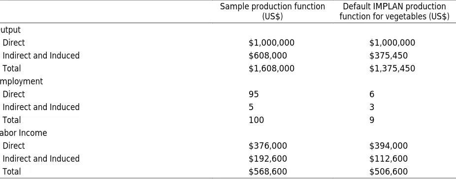
Using the modified production function, the model estimates that one million dollars in sales by the sample farmers will generate US$1.6 million in the regional economy (the 13-county study area) (Table 2). The same US$1 million in sales will support US$568,600 of labor income and 100 jobs. It should be noted, however, that the input-output model counts any job (even part-time) as one job. Study participants employed, on average, 2.7 peo-ple, all of whom worked part-time. Comparatively, using the default IMPLAN production function, US$1 million in sales will generate US$1.4 million in the local economy, support US$506,600 of labor income, and support nine jobs.
Table 2. Economic Contribution of US$1 Million in Sales, Sample Operations versus Default IMPLAN Production Function, in the 13-county Region
Sample production function
(US$) function for vegetables (US$)Default IMPLAN production Output
Direct $1,000,000 $1,000,000
Indirect and Induced $608,000 $375,450
Total $1,608,000 $1,375,450
Employment
Direct 95 6
Indirect and Induced 5 3
Total 100 9
Labor Income
Direct $376,000 $394,000
Indirect and Induced $192,600 $112,600
Total $568,600 $506,600
Discussion
The modified production function predicted a higher per-dollar economic impact than the default IMPLAN production function. This indicates that the small-scale, direct-to-consumer vegetable operations may have a greater impact on regional businesses than larger-scale, direct-to-wholesale operations, per dollar of output.
However, the quality of any economic impact analysis depends on the primary data that modifies or reflects the “ground truth” of an input-output model. The greatest difficulty in conducting this study was recruitment. In a 13-county area with an estimated 65 commercial vegetable producers, 11 agreed to participate. Even with the incentive of receiving a US$75 honorarium, business coaching, and custom data analysis for their farm, operators shied away, most often citing privacy issues. Researchers trying to collect valid and robust data are left to balance the trade-offs of personal interviews versus written or online surveys. While interviews, with both parties examining financial records together, may yield more accurate and detailed data from participants, they may seem too intrusive for some participants; further, interviews require a considerable investment of resources for researchers. A written or online survey may be viewed as more accessible and less intrusive, but given the complexity of farm financial data, may not yield the highest level of accuracy and detail.
The value of this research, despite the limited sample size, is two-fold. First, it demonstrates that changes to the production function to reflect local conditions can indeed affect relative impacts. The
results appear to indicate that small-scale, direct-to-consumer vegetable operators spend differently for inputs and spend more locally compared to the model default. These findings were consistent with those from Cornell’s study (Schmit et al., 2013; 2016). By following their recommendations for future research––namely a micro-level approach on a single production sector––our study reinforced their findings. Collecting the necessary data and incorporating them into an input-output model may help local food advocates better state their case that local food producers have significant and differential economic impact in their regions.
Second, this research project demonstrates how the fundamentals of the local food economics toolkit can be implemented in a region or sub-region of a state. It also shows how the collabora-tion of a project team (local produccollabora-tion specialists, farm-business management specialists, and an economic impact analyst) can modify the analysis to improve accuracy.
Acknowledgments
The authors would like to thank the full Extension team, farmer study participants, and advisory team which contributed to the research and made the project a success. The Extension team included Beth Berlin, Merritt Bussiere, Rob Holcomb, Randy Nelson, and our editor, Elyse Paxton. The advisory team included Lisa Baker, Arlene Jones, Kathy Zeman, and Molly Zins. Per our research agreement on confidentiality, farmer participants shall remain nameless, but you know who you are, and your contributions were greatest of all.
References
Becot, F., Conner, D., Imrie, D., & Ettman, K. (2016). Assessing the impacts of local hospital food procurement: Results from Vermont. Journal of Foodservice Management & Education, 10(1), 1–7. Retrieved from
https://www.fsmec.org/wp-content/uploads/2016/08/10-1-Becot.pdf
Benson, M., Niewolny, K., & Rudd, R. (2014). An evaluation of program, training, and resource needs of Virginia beginning farmers and ranchers: Virginia beginning farmer and rancher coalition program. Virginia Cooperative Extension. Retrieved from
https://vtechworks.lib.vt.edu/bitstream/handle/10919/56050/AEE-81.pdf
Conner, D. S., Knudson, W. A., Hamm, M. W., & Peterson, H. C. (2008). The food system as an economic driver: Strategies and applications for Michigan. Journal of Hunger and Environmental Nutrition, 3(4), 371–383.
https://doi.org/10.1080/19320240802528849
Crompton, J. L. (1995). Economic impact analysis of sports facilities and events: Eleven sources of misapplication. Journal of Sports Management, 9(1), 14–35. https://doi.org/10.1123/jsm.9.1.14
Henneberry, S. R., Whitacre, B., & Agustini, H. N. (2009). An evaluation of the economic impacts of Oklahoma farmers markets. Journal of Food Distribution Research, 40(3), 64–78. Retrieved from
https://econpapers.repec.org/article/agsjlofdr/99760.htm
Hughes, D. W., & Boys, K. A. (2015). What we know and don't know about the economic development benefits of local food systems. Choices, Q1. Retrieved from
http://choicesmagazine.org/choices-magazine/theme- articles/community-economics-of-local-foods/what-we-know-and-dont-know-about-the-economic-development-benefits-of-local-food-systems
Hughes, D. W., Brown, C., Miller, S., & McConnell, T. (2008). Evaluating the economic impact of farmers’ markets using an opportunity cost framework. Journal of Agricultural and Applied Economics, 40(1), 253–265.
https://doi.org/10.1017/S1074070800028091
Lazarus, W. F., Platas, D. E., Morse, G. W., & Guess-Murphy, S. (2002). Evaluating the economic impacts of an evolving swine industry: The importance of regional size and structure. Review of Agricultural Economics, 24(2), 458– 473. https://doi.org/10.1111/1467-9353.00109
Miller, R. E. & Blair, P. D. (2009). Input-Output analysis: Foundations and extensions (2nd ed.). New York, NY: Cambridge
University Press.https://doi.org/10.1017/CBO9780511626982
O’Hara, J. K., & Pirog, R. (2013). Economic impacts of local food systems: Future research priorities. Journal of Agriculture, Food Systems, and Community Development, 3(4), 35–42. https://doi.org/10.5304/jafscd.2013.034.003 Schmit, T. M., Jablonski, B. B. R., & Mansury Y. (2013). Impacts of local food system activities by small direct-to consumer producers
in a regional economy: a case study from upstate NY (Working Paper 2013-16). Charles H. Dyson School of Applied Economics and Management, Cornell University. Retrieved from
http://publications.dyson.cornell.edu/research/researchpdf/wp/2013/Cornell-Dyson-wp1316.pdf
Schmit, T., Jablonski, B., & Mansury, Y. (2016). Assessing the economic impacts of local food system producers by scale. Economic Development Quarterly, 30(4), 316–328. https://doi.org/10.1177/0891242416657156
Thilmany McFadden, D. T., Conner, D., Deller, S., Hughes, D., Meter, K. … Tropp, D. (2016, March). The economics of local food systems: A toolkit to guide community discussions, assessments, and choices. U.S. Department of Agriculture, Agricultural Marketing Service. Retrieved from https://www.rd.usda.gov/files/ILAMSToolkit.pdf
Tuck, B. Haynes, M., King, R., & Pesch, R. (2010). The economic impact of farm-to-school lunch programs: A Central Minnesota example. University of Minnesota Extension. Retrieved from
http://www.farmtoschool.org/Resources/Economic_Impact_of_F2S_Central_MN.pdf
Watson, P., Wilson, J., Thilmany, D., & Winter, S. (2007). Determining economic contributions and impacts: What is the difference and why do we care? The Journal of Regional Policy and Analysis, 37(2), 140–146. Retrieved from