http://www.sciencepublishinggroup.com/j/ijepe doi: 10.11648/j.ijepe.20170604.12
ISSN: 2326-957X (Print); ISSN: 2326-960X (Online)
Research/Technical Note
Particle Swarm Optimization Based Optimal Reactive Power
Dispatch for Power Distribution Network with Distributed
Generation
Khine Zin Oo, Kyaw Myo Lin, Tin Nilar Aung
Power System Research Unit, Department of Electrical Power Engineering, Mandalay Technological University, Mandalay, Myanmar
Email address:
[email protected] (K. Z. Oo), [email protected] (K. M. Lin), [email protected] (T. N. Aung)
To cite this article:
Khine Zin Oo, Kyaw Myo Lin, Tin Nilar Aung. Particle Swarm Optimization Based Optimal Reactive Power Dispatch for Power Distribution Network with Distributed Generation. International Journal of Energy and Power Engineering. Vol. 6, No. 4, 2017, pp. 54-60.
doi: 10.11648/j.ijepe.20170604.12
Received: June 21, 2017; Accepted: July 10, 2017; Published: August 11, 2017
Abstract:
Reactive power dispatch plays a main role in order to provide good facility secure and economic operation in the power system. Optimal reactive power dispatch (ORPD) is a nonlinear optimization problem and has both equality and inequality constraints. ORPD is defined as the minimization of active power loss by controlling a number of variables. Due to complex characteristics of ORPD, heuristic optimization has become an efficient solver. In this paper, particle swarm optimization (PSO) algorithm and MATPOWER toolbox are applied to solve the ORPD problem for distribution system with distributed generating (DG) plant. The proposed method minimizes the active power loss in a practical power system as well as determines the optimal placement of a new installed DG. The practical 41-bus, 6-machine power distribution network of Myingyan area is used to evaluate the performance. The result shows that the adjustment of control variables of distribution power network with a new DG gives a better approach than adjustment only the control variables without DG.Keywords:
Active Power Loss Minimization, Control Variables, DG, ORPD, PSO1. Introduction
The optimal reactive power dispatch (ORPD) is a sub problem of the optimal power flow calculation and has a significant influence on secure and economic operation of power systems. The controllable system quantities are the capacity of a new distributed generator, controlled voltage magnitude, reactive power injection from reactive power sources and transformer tapping [1]. The main objective of this paper is to minimize the active power loss by optimizing the control variables within their limits and to find the optimal placement of a new DG in distribution system.
Integrating of DG into distribution network already reduces power loss because some portion of the required current form upstream is substantially reduce which result lower loss through line resistance. Further reduction of loss can be achieved by intelligently managing reactive power from the installed DG [2].
Several conventional optimization algorithms [3] have been proposed to solve the ORPD problem such as linear programming, quadratic programming, and interior point method. Main problem associated with these conventional techniques is easily falling in local optimum solution. As the ORPD is nonlinear, evolutionary computation methods such as genetic algorithm (GA) [4], evolutionary programming (EP) and particle swarm optimization (PSO) [5] algorithm are best suitable to solve it.
The remaining of this paper is organized as follows: The mathematical model of optimal reactive power dispatch with DG is described in next section. DG reactive power supplying capability is then briefly discussed. In section 4, modified MATPOWER code utilizing PSO algorithm is provided to solve optimal reactive power dispatch problem of distribution network with DG. The 41-bus, 6-machine practical distribution network is challenged in this paper and the simulation results are discussed in Section 5. The last section provides the conclusions.
2. The Mathematical Model of Optimal
Reactive Power Dispatch
The goal of optimal reactive power dispatch [7-9] is to determine the optimum values of independent variables by optimizing a predefined objective function with respect to the operating bounds of the system. The ORPD problem can be mathematically expressed as a nonlinear constrained optimization problem as follows:
Minimize f(a,b) (1)
Subject to g(a,b)=0, equality constraint (2)
0, b)
h(a, ≤ inequality constraints (3)
where, a is vector of state variables, b is vector of control variables, f(a, b) is objective function, g(a, b) is different equality constraints set, h(a, b) is different inequality constraints set.
2.1. Variables
The control variables should be adjusted to satisfy the power flow equations. For the ORPD problem, the set for control variables can be formulated as [1, 2]:
[
G2 GNg G1 GNg C1 CNc 1 Nt]
T ...T T , ...Q Q , ...V V , ...P Pb = (4)
where, PG is real power output at the generator buses
excluding at the slack bus, VG is voltage magnitude of
generator buses, QC is shunt VAR compensation, T is tap
settings of transformer, Ng is no. of generator units, Nt is no. of tap changing transformers and Nc is no. of shunt VAR compensation devices, respectively.
There is a need of variables for all ORPD formulations for the characterization of the system. The state variables can be formulated as:
[
G1 L1 LNpq G1 GNg L1 LNL]
T ...S S , ...Q Q , ...V V , P
a = (5)
where, PG1 is real power generation at the slack bus, VL is
magnitude of voltage at load buses, QG is reactive power
generation of all generators, SL is transmission line loading,
Npq is no. of PQ buses and NL is no. of transmission lines, respectively.
2.2. Objective Function
The objective of the reactive power dispatch is to minimize the active power loss through controlling the capacity of reactive power control devices and the reactive power of DG. The expression can be described as follows:
∑
∑
∈ ∈ − + = = NL k ij j i 2 j 2 i k NL kkloss G (V V 2VVcosθ )
P
f (6)
where, NL is the number of transmission lines, Gk is the
conductance of the kth line, Vi and Vj are the voltage
magnitudes at the end buses i and j of the kth line and θ is ij
the voltage angle difference between buses i and j.
2.3. System Constraints
There are two ORPD constraints named inequality and equality constraints. These constraints are explained in the sections given below.
Equality Constraints: Minimization of objective function is subject to follow equality constraints. These constraints represent power flow active and reactive power balance equations.
∑
∈ = − + − − − NB j j i ij j i ij j i DiGi P V V[G cos(δ δ ) Bsin(δ δ )] 0
P (7)
∑
∈ = − + − − − NB j j i ij j i ij j i DiGi Q V V[Gsin(δ δ) Bcos(δ δ)] 0
Q
(8)
where, PG is the active power generated, QG is the reactive
power generated, PD is the active power demand, QD is the
reactive power demand, NB is total no. of buses, Gij and Bij are
the transfer conductance and susceptance between bus i and j.
Inequality Constraints: The inequality constraints are typically technical limitations of the power system devices in the network. Inequality constraints represent the system operating limits as: [3-4].
(a)Generator Constraints: Generator voltages and generated reactive power outputs are limited to as follows:
max Gi Gi min
Gi V V
V ≤ ≤ (9)
max Gi Gi min
Gi Q Q
Q ≤ ≤ (10)
where, i=1, 2, 3,…., Ng. Ng is no. of generator buses. (b)Transformer Constraints: Transformer tap settings are
restricted to as follows:
max i i min
i T T
T ≤ ≤ (11)
where, i=1, 2, 3,…., Nt. Nt is no. of tap setting transformers. (c)Shunt VAR Compensator Constraints: Shunt VAR
compensation limits are as follows:
max ci ci min
ci Q Q
where, i=1, 2, 3,…, Nc. Nc is no. of shunt compensation buses.
The control variables are self-constrained variables. In this reactive power dispatch problem, the inequality constraints are incorporated as penalty terms into the objective function in (6). The fitness function for above reactive power dispatch problem is generalized as follows:
∑
∑
∈ ∈ − + − + = Npqi i Nt
2 lim i i Ti 2 lim i i
Vi(V V ) (T T )
f
F λ λ
+
∑
∈ − Ng i 2 lim Gi Gi Gi(Q Q )λ (13)
where, λVi is the penalty multiplier for voltage limit, λTi is
the penalty multiplier for transformer tap setting limit and
Gi
λ is the penalty multiplier for generated reactive power limit respectively. Penalty multipliers are large positive constants for minimum deviation in these inequality constraints.
Limiting values of V , T and Q are defined as follows: < > = min i i min i max i i max i lim i V V ; V V V ; V
V (14)
< > = min i i min i max i i max i lim i T T ; T T T ; T
T (15)
< > = min Gi Gi min Gi max Gi Gi max Gi lim Gi Q Q ; Q Q Q ; Q
Q (16)
3. Reactive Power Supply Capability of
Distributed Generation
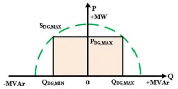
DG connected to electrical grid through power electronic converter can be set to inject reactive power by changing its operating power factor or increasing its reactive current output. How much reactive power can be supplied by DG unit depends on its active power set point. The diagram illustrating reactive power capability is shown in Figure 1. If DG active power is set close to its rated apparent power rating, capacitive or inductive reactive power range that can be supplied is small. Reactive supply capability of DG can be increased by reducing its active power generation. If active power set point is reduced, more reactive supply is guaranteed [10].
Figure 1. Apparent, active and reactive power from DG point.
Even though the amount of reactive power that can be supplied by DG is limited and is not enough to supply the entire reactive power requirement, this corrective action in consequence can minimize the power losses inside the distribution network. As DG unit will be integrated into distribution network depending on the location, reactive power amount required from DG unit will be varied in different operating conditions. In finding optimal reactive power, optimization algorithm such as particle swarm optimization is required [11].
Not all DG technology is suitable to control reactive power continuously. For an example, DG from intermittent resources such as Photovoltaic is not reliable because the required services probably cannot be delivered when it is needed. The technologies of synchronous generator based DG, micro turbine generation system and fuel cell can fit this requirement. These technologies are available commercially and capable to provide active power and other services such as reactive current injection when required.
4. A Technique of Particle Swarm
Optimization Combined with
MATPOWER Toolbox
Power system optimization problems are more complication and diversity when additional constraints are considered. The heuristic algorithm optimization is required in finding the optimal settings of control variables including voltage magnitude of a new DG. In this paper, the technique of applied MATPOWER into a particle swarm optimization (PSO) algorithm is contributed to solve ORPD problem integrating a DG.
4.1. MATPOWER
MATPOWER [12] is a powerful MATLAB programming package for power flow and optimal power flow solving. The biggest advantage of MATPOWER is its easiness to use and modify the original code. MATPOWER process can be applied into particle swarm optimization in terms of loss reduction in power system. The process of MATPOWER comprises of three steps as follows:
Step 1:
Input file, the power system data such as bus data, branch data and generator data will be read for next steps.
Step 2: Calculate the power flow by Newton-Raphson method.
Step 3: Display all results.
4.2. Particle Swarm Optimization
The particle swarm optimization algorithm (PSO) was discovered by James Kennedy and Russell C. Eberhart in 1995 [13, 14]. This algorithm is inspired by simulation of social psychological expression of birds and fish. PSO includes two terms pbest and gbest. The concept of modification of a
of each particle is updated over the course of iteration from these mathematical equations:
+ − +
=
+ w .v c.rand.(pbest x )
v k
id id 1 1 k id k 1 k
id (17)
) x .(gbest .rand
c k
id d 2
2 −
where, c1, c2 are acceleration constants, k is the current
iteration number.
The first part of (17) provides momentum to the particles. It provides diversification to the particles in search procedure. The inertia weight constant of the particles which controls the exploration of the search space, given by:
iter * iter
w w w
w max
min max max
k = − −
(18)
The second and third parts of (17) are known as cognitive component and social component respectively. These components provide attraction towards best ever position and attraction towards best previous performance of neighborhood respectively. ‘iter’ is the number of iterations to be performed. Each particle’s position is updated as (19).
1 k id k id 1 k
id x v
x + = + + (19)
Figure 2. Concept of modification of a search point.
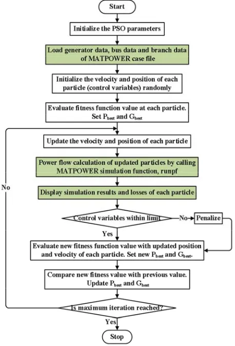
4.3. Step by Step Procedures of PSO Algorithm Combined with MATPOWER Toolbox for ORPD
In the ORPD problem, the elements of the solution consist of all control variables, namely, generator bus voltages, the transformer tap setting and the reactive power generation. These variables are representing continuous variables in the PSO population. The fitness function of ORPD problem presented in this paper is to minimize the total power loss. For each individual, the equality constraints given by (7) and (8) are satisfied by using MATPOWER toolbox.
Step by step procedures to implement the optimal reactive power dispatch problem using PSO combined with MATPOWER toolbox are as follows:
Step 1:
Initialization of PSO parameters. Load case information: the system data; generator data, bus data and branch data are saved in MATPOWER case file.
Step 2: Initialize various particles (control variables) values randomly.
Step 3: Find fitness value of fitness function and save pbest and gbest values.
Step 4: Update the velocity and position of each particle using (17) and (19).
Step 5:
Call MATPOWER simulation function ‘runpf’ to run power flow updated particles’ positions and velocities.
Step 6:
Display simulation results and loss of each particle after power flow calculation using MATPOWER.
Step 7:
Check whether the inequality constraints violates the limit or not at the end of power flow. If the solution exceeds the limits, penalize the violations.
Step 8: Find new fitness value of fitness function using updated particle position and velocity.
Step 9:
Compare new fitness value with previous value. If the new fitness value obtained is better than the previous value, update new pbest and gbest.
Step 10: Repeat above procedure from step 4 for max no. of iterations.
The flow chart of the PSO algorithm combined with MATPOWER toolbox for ORPD is illustrated in Figure 3.
5. Simulation Results and Discussion
5.1. Case Study System Network
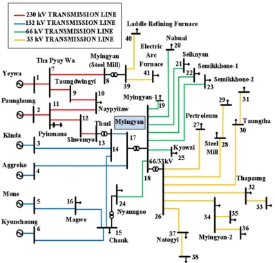
To demonstrate the effectiveness of the proposed PSO based algorithm for reactive power dispatch, a practical 41-bus distribution test system is used as shown in Figure 4. The distribution system is extracted from 132/66/33 kV Myingyan substation in Myingyan area of Myanmar. The voltage levels of the test system are 230 kV, 132 kV, 66 kV and
33 kV. This system has 6 generating stations, 36 load buses, 41 branches, 5 transformers, and 1 shunt reactive power compensator at bus 11. The incoming line of Myingyan substation is 132 kV line. There are 19 outgoing lines (66 kV and 33 kV lines). Yeywa (bus 1) is taken as the slack bus and other five generators are located at bus 2, 3, 4, 5 and 6 respectively. The evident features of the simulation results are also discussed in this section.
Figure 4. Practical 41-bus test system.
The initial operating conditions for the proposed method are given as follows for 100 MVA base. The total load of the test system is 252.92 MW and 130.58 MVAr. MATPOWER toolbox is used to calculate the power flow of practical 41-bus distribution system. Before optimization, the total real and reactive power loss of the entire system is 15.969 MW and 32.87 MVAr, respectively.
5.2. Parameters of PSO Based ORPD
To successfully implement the proposed method for ORPD problem, the setting limits of reactive power control variables are shown in Table 1. The bus voltage magnitudes are maintained within 0.9 to 1.1 p.u. Table 2 shows the penalty
factors of the fitness function used in (13). The basic parameters of PSO algorithm are shown in Table 3.
Table 1. Variable Limits (p.u).
Reactive Power Generation Limits (MVAr)
Bus 1 2 3 4 5 6
QGmax 130 70 10 25.3 17.8 20
QGmin -130 -70 -10 -25.3 -16.8 -10
Voltage and Tap Setting Limits (p.u)
Vimin Vimax Timin Timax
0.9 1.1 0.95 1.05
Shunt VAR Compensation Limits (MVAr)
Bus Qcmin Qcmax
Table 2. Optimal Penalty Settings.
V i
λ λTi λGi
25500 10000 1000
Table 3. Basic Parameters of PSO for ORPD.
Sr. No Parameters Value
1 Population size 40
2 Maximum inertia weight 0.9
3 Minimum inertia weight 0.4
4 Acceleration constants [c1, c2] [2.05, 2.05]
5 Maximum number of iterations 200
6 Random number [0, 1]
5.3. Testing Scenarios
Two scenarios were considered to show the effectiveness of the proposed method to control reactive power on practical 41-bus distribution system. The conventional PSO algorithm has been implemented in MATLAB programming language incorporated with MATPOWER package, and numerical tests are carried out on a core i5, 2.20 GHz, 4 GB RAM computer.
Scenario 1: Optimal reactive power dispatch without new DG and
Scenario 2: Optimal reactive power dispatch with new DG and finding optimal placement of a new DG.
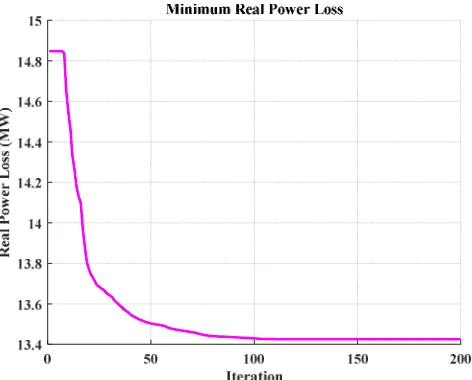
Scenario 1: Optimal reactive power dispatch without new DG.
Figure 5 shows the optimization process of the proposed method without installing a new DG. At the beginning of the process, optimal active power loss is about 15 MW. As the particles continually update their positions towards the best solution, the real power loss keeps decreasing. After 160 iterations, no obvious improvement can be observed. Finally, the total power loss of the system converges to 13.4251 MW. The total CPU time is about 622.114 sec.
Figure 5. Loss reduction process without new DG.
The voltage profile of case study network after optimization using particle swarm optimization is shown in Figure 6. It can be observed that the voltages at each bus are maintained
within their acceptable limits.
Figure 6. Voltage profile after optimization.
Table 4 demonstrates the comparison of the original network base case solution with optimization using PSO without a new DG. The total active power loss value obtained initially was 15.969 MW and it has been reduced by the proposed PSO method to 13.4251 MW. The best control variables after optimization for scenario 1 are presented in this table. It can be clearly seen that all control variables are within their specific ranges.
Table 4. Comparison of Control Variables for Scenario 1.
Control Variables Min Max Base Case PSO
Generator Voltage Magnitude
VG1 0.9 1.1 1.0600 1.1000
VG2 0.9 1.1 1.0000 1.0432
VG3 0.9 1.1 1.0000 1.0214
VG4 0.9 1.1 1.0100 0.9932
VG5 0.9 1.1 1.0000 0.9909
VG6 0.9 1.1 0.9500 0.9836
Transformer Tap Setting
T8-39 0.95 1.05 0.9301 0.9841
T13-14 0.95 1.05 0.9720 0.9996 T15-24 0.95 1.05 0.9003 0.9911 T17-18 0.95 1.05 0.9780 0.9829 T18-26 0.95 1.05 0.9320 0.9560 Shunt VAR
Compensation Qc11 0 10 6.0000 6.5505
Active Power Loss - - 15.969 MW 13.4251
MW
Scenario 2: Optimal placement of a new DG.
The second scenario is about adding a new DG to the practical 41-bus system and then optimizes the reactive power of the system by using the proposed approach. A direct-derive synchronous generator and gas turbine is selected as the new DG. Its rated power is 2050 kW which can deliver 1.2 MVAr and -1.0 MVAr reactive powers. The optimal placement of a new DG in 33 kV Myingyan distribution network is determined in this scenario.
when DG is installed on various buses of 33 kV Myingyan distribution network is illustrated in Figure 7.
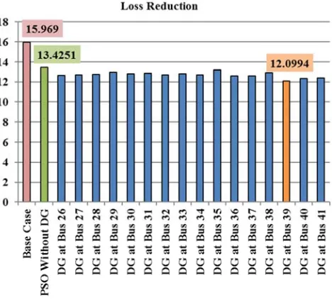
Figure 7. Comparison of loss reduction.
It can be seen that optimization with a new DG can further reduce the active power loss than optimization using PSO without DG. After integrating a new DG on bus 39, the total active power loss can be reduced to minimum 12.0994 MW. The optimal placement of a new DG is on bus 39. Figure 8 shows the optimal loss reduction process of the proposed method when a small gas turbine is installed on bus 39. The initial real power loss of the system is at about 16.5 MW. The particles start to converge after conducting 130 iterations. Finally, the total power loss of the system is 12.0994 MW. The total CPU time is 651.403 sec.
Figure 8. Loss reduction process when new DG is installed on bus 39.
Figure 9 shows the comparison of the active power loss of the base case, optimization without DG and optimization with new DG on bus 39. It can be observed that the active power loss on most of the branches is significantly reduced after optimization with a new DG.
Figure 9. Comparison of active power loss.
The results from Table 5 show that the optimal settings of control variables to get minimum active power loss when a new DG is installed on bus 39. There are 13 control variables which optimize reactive power and the proposed method succeeds in keeping all control variables within their limits. The total active power loss after optimization with a new DG is 12.0994 MW.
Table 5. Optimal Results of Control Variables for Scenario 2 with DG.
Control Variables Min Max With New DG on Bus 39
Generator Voltage Magnitude
VG1 0.9 1.1 1.1000
VG2 0.9 1.1 1.0411
VG3 0.9 1.1 1.0190
VG4 0.9 1.1 0.9995
VG5 0.9 1.1 0.9992
VG6 0.9 1.1 0.9810
VDG, 39 0.9 1.1 1.0655
Transformer Tap Setting
T8-39 0.95 1.05 0.9803
T13-14 0.95 1.05 0.9814 T15-24 0.95 1.05 1.0148 T17-18 0.95 1.05 1.0187 T18-26 0.95 1.05 1.0280 Shunt VAR
Compensation Qc11 0 10 6.5845
Active Power Loss - - 12.0994 MW
Table 6. Optimal Reactive Power Output of Generators.
No QMIN QOUT QMAX
QG1 -130 14.491 130
QG2 -70 54.807 70
QG3 -10 7.487 10
QG4 -25.3 19.185 25.3
QG5 -16.8 8.817 17.8
QG6 -10 14.491 20
QDG, 39 -1 30.783 1.2
6. Conclusion
In this paper, combined technique of particle swarm optimization algorithm with MATPOWER toolbox is applied to solve reactive power dispatch problem and to determine the optimal placement of new installed DG in existing system. The performance of the proposed technique has been tested on the 41-bus distribution system and compared the simulation results without and with DG. It can be observed that reactive power dispatch approach for distribution system with a distributed generation can further reduce the active power loss than without DG. The benefit of lower active power loss obtained will provide better economic dispatch and secure operation in power system.
References
[1] W. Ongsakul and D. N. Vo, “Artificial Intelligence in Power System Optimization,” Taylor & Francis Group, LLC, 2013. [2] L. Shengqi, Z. Lilin, L. Yongan, and H. Zhengping, “Optimal
Reactive Power Planning of Radial Distribution Systems with Distributed Generation,” Third International Conference on Intelligent System Design and Engineering Applications, 2013. pp. 1030-1033.
[3] T. Sharma, A. Yadav, S. Jamhoria, and R. Chaturvedi, “Comparative Study of Methods for Optimal Reactive Power Dispatch,” Electrical and Electronics Engineering, vol. 3, no. 3, 2014, pp. 53-61.
[4] K. Naima, B. Fadela, C. Imene, and C. Abdelkader, “Use of Genetic Algorithm and Particle Swarm Optimization Methods for the Optimal Control of the Reactive Power in Western Algerian Power System,” Energy Procedia 74, 2015, pp. 265-272.
[5] Y. Amrane and M. Boudour, “Optimal Reactive Power Dispatch Based on Particle Swarm Optimization Approach Applied to the Algerian Electric Power System,” IEEE 2014
11th International Multi-Conference on Systems, Signals and Devices – Castelldefels-Barcelona, Spain, 2014.
[6] Kittavit Buayai, Kittiwut Chinnabutr, Prajuap Intarawong, and Kaan Kerdchuen, “Applied MATPOWER for Power System Optimization Research,” Energy Procedia, vol. 56, 2014, pp. 505-509.
[7] A. Ghasemi, and A. Tohidi, “Multi Objective Optimal Reactive Power Dispatch Using a New Multi Objective Strategy,” Electrical Power and Energy Systems, vol. 57, 2014, pp. 318-334.
[8] T. Malakar, and S. K. Goswami, “Active and Reactive Power Dispatch with minimum control movement,” Electrical Power System Research, vol. 44, 2013, pp. 77-87.
[9] Y. Li, Y. Wang, and B. Li, “A Hybrid Artificial Bee Colony assisted Differential Evolution Algorithm for Optimal Reactive Power Flow,” Electrical Power System Research, vol. 52, 2013, pp. 25-33.
[10] M. Zamri Che Wanik, I. Erlich, and A. Mohamed, “Intelligent Management of Distributed Generators Reactive Power for Loss Minimization and Voltage Control,” IEEE, 2010, pp. 685-690.
[11] U. Leeton, T. Ratniyomchai and T. Kulworawanichpong, “Optimal Reactive Power Flow with Distributed Generating Plants in Electric Power Distribution Systems,” International Conference on Advances in Energy Engineering, 2010. [12] J. Zhu, R. D. Zimmerman and C. E. Murillo-Sanchez,
“MATPOWER 5.1 User’s Manual,” March 20, 2015.
[13] N. K. Patel, and B. N. Suthar, “Optimal Reactive Power Dispatch Using Particle Swarm Optimization in Deregulated Environment,” International Conference on EESCO, 2015. [14] S. Pandya, and R. Roy, “Particle Swarm Optimization Based