Article
1
Duality Based Risk Mitigation Method for
2
Construction of Joint Hydro-Wind Coordination
3
Short-Run Marginal Cost Curves
4
Perica Ilak *, Ivan Rajšl, Josip Đaković and Marko Delimar
5
Department of Energy and Power Systems, University of Zagreb Faculty of Electrical Engineering and
6
Computing, Unska 3, Zagreb HR-10000, Croatia;
7
E-Mails: [email protected]; [email protected]; [email protected]; [email protected]
8
* Correspondence: [email protected]; Tel.: +385-1-6129-693
9
Abstract: This study analyses the short-run hydro generation scheduling for the wind power
10
differences from the contracted schedule. The approach for construction of the joint short-run
11
marginal cost curve for the hydro-wind coordinated generation is proposed and applied on the real
12
example. This joint short-run marginal cost (SRMC) curve is important for its participation in the
13
energy markets and for economic feasibility assessment of such coordination. The approach credibly
14
describes the short-run marginal costs which this coordination bears in “real life”. The approach is
15
based on the duality framework of a convex programming and as a novelty combines the shadow
16
price of risk mitigation capability and the water shadow price. The proposed approach is formulated
17
as a stochastic linear program and tested on the case of the Vinodol hydropower system and the
18
wind farm Vrataruša in Croatia. The result of the case study is a family of 24 joint short-run marginal
19
cost curves.
20
Keywords: Convex programming; Wind power, Hydropower; Risk mitigation; CVaR; Short-run
21
marginal cost curve
22
23
Nomenclature
24
Symbols
𝑐′ Short-run marginal cost function (€/MW∙h).
𝑑 Difference between forecasted 𝑌 and actual wind generation 𝑦𝑤 (MW). 𝑑+ Positive wind difference (MW).
𝑑− Negative wind difference (MW). 𝑒 Natural water inflow (MW).
𝐹𝛼 Special function used for risk shaping of CVaR (€). 𝑔 Net outflow of hydro generation (MW)
𝐼 Hourly revenue (€).
𝑘𝑆𝑡 Maximal capacity of reservoir (MW∙h).
𝑘𝑅𝑚 Parameter used for risk exposure reduction in risk shaping procedure (€). 𝑘𝑇𝑢 Hydro turbine maximal capacity (MW).
𝑘𝑇𝑢𝑤 Wind turbine maximal capacity (MW). 𝑛𝑆𝑡 Minimal capacity of reservoir (MW∙h).
𝑛𝑇𝑢 Hydro turbine minimal capacity (MW). 𝑛𝑇𝑢𝑤 Wind turbine minimal capacity (MW).
𝑠 Energy stock, amount of water in reservoir in t, (MW∙h). 𝑠0 Energy stock at the beginning of planning interval (MW∙h)
𝑠𝑇 Energy stock surplus or deficit at the end of planning interval (MWh) 𝑦 Hydro generation (MW).
Y Contracted wind generation (MW). 𝑦𝑤 Actual wind generation (MW). Greek
𝛼 Percentile used for the CVaR where 1-𝛼 defines the worst events (%). 𝛿 Shadow prices associated with constraint of CVaR’s helping variable 𝜂 (€).
𝜀 Shadow prices associated with CVaR’s hourly revenue constraint. 𝜁 The decision variable which defines the Value at Risk (€).
𝜂 Variable used for obtainment of the CVaR (€).
𝜅𝑇𝑢 Shadow price of hydro generation maximum capacity (€/MW∙h).
𝜅𝑆𝑡 Shadow price of reservoir maximum capacity (€/MW∙h).
λ Shadow price of energy stock surplus/deficit at the end of operation (€/MW∙h).
𝜈Tu Shadow price of hydro generation minimum capacity (€/MW∙h). 𝜈𝑆𝑡 Shadow price of reservoir minimum capacity (€/MW∙h).
𝜉 Shadow price of risk mitigation capability (dimensionless).
𝜋 Price of electricity (€/MW∙h).
𝜓 Shadow price of water (€/MW∙h).
Spaces
[0, 𝑇] Planning interval, subspace of the real line 𝑡 ∈ [0, 𝑇] ⊂ ℝ.
1. Introduction
25
In this paper the hydro-wind coordination is formulated as a hydro-economic river basin model
26
(HERBM). The coordination assumes that hydro generation is scheduled for firming wind generation.
27
In other words, the short-run hydro generation is scheduled for the wind power differences from the
28
contracted schedule. This wind power difference from contracted schedule impacts the short-run
29
marginal cost curve of the hydro generation curve in the coordination [1]. Generally, a short-run
30
marginal cost curve of a hydro generation is obtained from the water shadow price and as such is
31
important for economic feasibility assessment of the coordination. In this paper, the joint short-run
32
marginal cost curve for electricity generation of hydro-wind coordinated generation is obtained. To
33
obtain these joint short-run marginal curves, the primal problem and its dual are formulated as
34
convex optimization problems. The primal problem is defined as a short-run revenue maximization
35
problem, while the dual problem minimizes the usage costs of the limited resources (hydro and wind
36
turbine capacity, reservoir capacity, water inflow resource, wind difference resource, risk mitigation
37
capability).
38
This paper is based on the pioneering works [2-3] which systematically address the problem of
39
the short run profit maximization of the hydro and the pumped storage units using continuous
40
functions and [4] where method for the contraction of short-run marginal cost curves for hydro
41
generation is given. These works are based on the ideas of conjugate duality and optimization [5].
42
The issue of hydro-wind coordination is addressed extensively and among the most significant are
43
the following papers. The sizing method for the pumped hydro storage which uses the wind power
44
surplus is presented in [6]. A methodology for increasing profits of a generation company that owns
45
wind and pumped-storage plants while accounting the wind power uncertainty is presented in [7].
46
In [8] the problem of introduction of the new pumped-storage station to the existing hydropower
47
system owned by a new subject is addressed. In [9] a combined strategy for bidding and operating in
48
a power exchange is presented. It considers the combination of a wind generation company and a
49
a hydro generating unit on the wind farm revenue in a pool-based electricity market, considering the
51
uncertainty of wind power prediction. The [11] proposes methodology that can reflect different risk
52
profiles of decision makers in wind–hydro-thermal coordination and in [12] a joint operation between
53
a wind farm and a hydro-pump plant is proposed to decrease costs of wind farm imbalances.
54
This paper will complement these studies by tackling the issue of contraction of joint short-run
55
marginal cost curves for the hydro-wind coordination. Obtaining a joint short-run marginal cost
56
curves for a hydro-wind coordination is hard issue due to facts that electricity generation from the
57
hydro-wind coordination is: a) storable and; b) has a negligible direct generation cost. Therefore,
58
usual approach (first derivative by output of the total cost function) for obtainment of short-run
59
marginal cost curves is not sufficient in this case. This issue was not tackled until the fundamental
60
works [4] where issue of constructing short-run marginal cost curve for a hydro producer is analyzed
61
and [1] where the impact of a wind power difference from contracted schedule on the water shadow
62
price is analyzed. This paper, as an extension of the research done in [1] and [4], contributes with the
63
systematic approach for construction of the joint short-run marginal cost curves for a hydro-wind
64
coordination.
65
Therefore, this research contributes with the approach based on duality method of convex
66
programming for construction of the joint short-run marginal cost curves for electricity generation of
67
a hydro-wind coordination which as a novelty combines: i) a shadow price of risk mitigation
68
capability, ξ; ii) and a water shadow price, ψ. The approach enables quantification of hourly cost of
69
risk mitigation through the shadow price of risk mitigation capability, ξ. The proposed approach is
70
formulated as a stochastic linear program and is easy to implement in various optimization problems.
71
The approach is tested on the case study of Vinodol hydropower system and the wind farm Vrataruša
72
in Croatia resulting in a family of 24 joint short-run marginal cost curves. The cost of risk mitigation
73
is also provided. To implement risk mitigation, the CVaR risk measure is used, which enables
74
measurement and limitation of extreme financial losses. It is a coherent risk measure [14-18] which
75
means that it satisfies properties of monotonicity, sub-additivity, positive homogeneity and
76
translational invariance. For the risk measure which satisfies these properties it is said that it describes
77
well a real life occurring risks. The properties of sub-additivity and positive homogeneity can be
78
replaced by property of convexity which is important when implementing in convex optimization
79
problems in order not to undermine its convexity1.
80
Besides the CVaR, the second important term is the water shadow price. The idea behind the water
81
shadow price is that generation of 1 MW∙h in particular hour means not being able to produce that 1
82
MW∙h in other future hours (it is important to notice that the water shadow price can also be regarded
83
as an opportunity cost of water generation in particular hour). Generally, the shadow price is equal
84
to the marginal utility of relaxing particular constraint or marginal cost when constraint is
85
strengthened. In this case, generation of 1 MW∙h means strengthening water balance constraint by 1
86
MW∙h, in particular hour. Therefore, by definition, a water shadow price can be regarded as a
87
marginal cost which makes it appropriate for construction of short-run marginal cost curves2. In
88
fundamental works [20,21] the water shadow price is assumed to be constant over the planning
89
period [0, T]. For more realistic approach the water shadow price should change over the planning
90
period, such as in [1-4], every time when reservoir limits are reached, which is also assumed here.
91
In Chapter II, the short-run dual for valuing limited hydro-wind generation resources is set as
92
the double infinite linear programming problem. The dual is reformulated for shadow pricing of
93
water in the coordinated hydro-wind generation. The wind power difference from contracted
94
schedule and CVaR are implemented in the dual problem through the duality framework of convex
95
1 See Corollary 11 in [18] for more about convexity of CVaR.
programming. In the Chapter III cascaded hydropower system Vinodol is carefully modeled as the
96
HERBM [22,23] and the wind farm Vrataruša power difference is implemented within it. The results
97
are presented and discussed in the same Chapter. In the Chapter IV conclusions are given.
98
2. Construction of the joint short-run marginal cost curve
99
The primal problem is a short-run profit maximization problem shown in Eqs. (1) - (14). To
100
achieve strong duality, the primal problem must be convex and needs to satisfy Slater's condition. The
101
primal problem used here is a linear program, i.e. it is convex and it satisfies Linearity constraint
102
qualification which is sufficient condition for strong duality. Strong duality is important here since it
103
implies that the duality gap, i.e. difference between the primal and dual solutions is zero. The dual
104
to the primal problem is shown in Eqs. (15) - (21) and is used for the construction of the joint
short-105
run marginal cost curves for the hydro-wind coordination.
106
For hydro generation, it is assumed that minimal and maximal reservoir capacities are 𝑛𝑆𝑡
107
and 𝑘𝑆𝑡 (Eq. (6)) and are measured in terms of energy (MW∙h) same as water stock measured which
108
is stored at no cost. The natural water inflow 𝑒 into the reservoir is measured over [0, 𝑇] in MW.
109
Wind power difference 𝑑 is measured over [0, 𝑇] in MW and can obtain positive 𝑑+ and
110
negative 𝑑−values (Eq. (12)). The units are MW due to continuous-time dating (see Eq. (2) and Eq.
111
(16)). It is defined as the difference between generated wind power and power indicated in contracted
112
schedule. The hydro turbine operating range in Eq. (4) is limited by: its minimal and maximal
113
capacity 𝑛𝑇𝑢 and 𝑘𝑇𝑢 measured in MW; the positive 𝑑+ and the negative 𝑑− wind difference. The
114
performance curve of the hydro generation is considered linear and the head is fixed over the
115
planning interval [0, 𝑇] ∈ ℝ. The goal function (Eq. (2)) maximizes the expected revenue obtained
116
from day-ahead energy market over the planning interval [0, 𝑇] which is multiplied with the
117
probability 𝑃(𝐴) of event 𝐴. The 𝑦 is the hydro generation measured in MW and 𝜋 is the
118
electricity price measured in €/MW∙h since of continuous-time dating. The decision variables in Eq.
119
(3), over which the goal function (Eq. (2)) is optimized, consist of the electricity generation variable
120
𝑦 and (𝜁, 𝜂) which are decision variables associated with CVaR risk measure.
121
According to the Theorem 14 in [18] the CVaR can be implemented in the optimization problem
122
as a goal function, a constraint or both. Since the goal function is predefined here, then CVaR is
123
implemented with Eq. (7) - (9). The risk mitigation is done through risk shaping of the special function
124
𝐹𝛼 with the parameter 𝑘𝑅𝑚, according to the Theorem 16 in [18]. The 𝑘𝑅𝑚 is measured in monetary
125
units (€) and represents the minimum desired level of revenue the owner expect in worst 1 − 𝛼
126
outcomes (usually 5%, where 𝛼 = 95%) and is part of input data (Eq. (1)). The decision variable 𝜁 in
127
Eq. (3) defines the Value at Risk (VaR) measure and 𝜂 is a variable used for determining hourly
128
revenue in worst case events, both these are used for obtainment of the CVaR3. The electricity price
129
𝜋 is expressed in €/MW∙h. The 𝑠0 defines the energy stock at the beginning of planning interval in
130
MW∙h and 𝑠𝑇 energy stock surplus or deficit at the end of planning interval in MW∙h. Both
131
parameters are the result of the middle-term HERBM optimization and part of the input data (Eq.
132
(1)). The input data is same for primal (Eq. (1)), and dual problem (Eq. (15)). The 𝑔 in Eq. (10) defines
133
the net outflow from the reservoir measured over [0, 𝑇] in MW. When net outflow 𝑔 is integrated
134
over time (Eq. (5)) it equals amount of water left at the end of planning horizon, T, which should be
135
above or equal to the predefined level, 𝑠𝑇. To preserve clarity, in depth analysis of the primal and
136
dual problems is provided in the comments section. Therefore, a primal problem is (the variables
137
denoted after the “;” in equations are the dual variables/shadow prices associated with the
138
constraints):
139
Given
(𝜋; 𝑛𝑇𝑢; 𝑘𝑆𝑡, 𝑛𝑆𝑡, 𝑘𝑇𝑢, 𝑠0, 𝑠𝑇; 𝑑, 𝑒, 𝑘𝑅𝑚) (1)
Maximize
∫ ∑ 𝑃(𝐴) ∙ 𝜋(𝑡, 𝐴) ∙ 𝑦(𝑡, 𝐴) 𝐴∈ℱ𝑡
dt 𝑇
𝑡=0
(2)
Over
(𝜁, 𝜂, 𝑦) (3)
Subject to
𝑛𝑇𝑢+ 𝑑+(𝑡) ≤ 𝑦(𝑡, 𝐴) ≤ 𝑘𝑇𝑢 + 𝑑−(𝑡) ; 𝜅𝑇𝑢(𝑡, 𝐴), 𝜈Tu(𝑡, 𝐴) (4)
∫ 𝑔(𝑡, 𝐴) 𝑇
𝑡=1
dt ≤ 𝑠𝑇 ; 𝜆(𝐴) (5)
𝑛𝑆𝑡≤ 𝑠0− ∫ 𝑔(𝜏, 𝐴) 𝑡
𝜏=1
dτ ≤ 𝑘𝑆𝑡 ; 𝜈St(𝑡, 𝐴), 𝜅St(𝑡, 𝐴) (6)
𝜁(𝑡) − 𝐼(𝑡, 𝐴) − 𝜂(𝑡, 𝐴) ≤ 0 ; 𝜀(𝑡, 𝐴) (7)
𝜂(𝑡, 𝐴) ≥ 0 ; 𝛿(𝑡, 𝐴) (8)
𝐹𝛼(𝜂(𝑡, 𝐴), 𝜁(𝑡)) ≥ 𝑘𝑅𝑚 ; 𝜉(𝑡) (9)
Where
𝑔(𝑡, 𝐴) ∶= 𝑦(𝑡, 𝐴) − 𝑑(𝑡, 𝐴) − 𝑒(𝑡, 𝐴) (10)
𝐼(𝑡, 𝐴) ≔ 𝜋(𝑡, 𝐴) ∙ 𝑦(𝑡, 𝐴) (11)
𝑑(𝑡) ∶= 𝑑−(𝑡) + 𝑑+(𝑡) (12)
|𝑑−(𝑡)| ∧ 𝑑+(𝑡) = 0 (13)
𝐹𝛼(𝜂(𝑡, 𝐴), 𝜁(𝑡)) ∶= 𝜁(𝑡) − 1
1 − 𝛼∑ 𝑃(𝐴) ∙ 𝜂(𝑡, 𝐴) 𝐴∈ℱ
(14)
And its dual:
(𝜋; 𝑛𝑇𝑢; 𝑘𝑆𝑡, 𝑛𝑆𝑡, 𝑘𝑇𝑢, 𝑠0, 𝑠𝑇; 𝑑, 𝑒, 𝑘𝑅𝑚) (15)
Minimize
∫ ∑ (𝑘𝑇𝑢+ 𝑑−(𝑡, 𝐴)) ∙ 𝜅𝑇𝑢(𝑡, 𝐴) − (𝑛𝑇𝑢+ 𝑑+(𝑡, 𝐴)) ∙ 𝜈𝑇𝑢 𝐴∈ℱ𝑡
(𝑡, 𝐴) + (𝑘𝑆𝑡− 𝑠0) ∙ 𝜅𝑆𝑡(𝑡, 𝐴) 𝑇
0
+ (𝑠0− 𝑛𝑠𝑡) ∙ 𝜈𝑆𝑡(𝑡, 𝐴) + (𝑒(𝑡) + 𝑑(𝑡)) ∙ 𝜓(𝑡, 𝐴) 𝑑𝑡 + ∑ 𝑠𝑇∙ 𝜆(𝐴) 𝐴∈ℱ𝑡
+ ∫ 𝑘𝑅𝑚(𝑡) ∙ 𝜉(𝑡) 𝑑𝑡 𝑇
0
(16)
Over
(𝜅𝑇𝑢, 𝜈Tu, 𝜅𝑆𝑡, 𝜈𝑆𝑡, 𝜆, 𝜀, 𝛿, 𝜉) (17)
Subject to
𝜓(𝑡, 𝐴) + 𝜅𝑇𝑢(𝑡, 𝐴) − 𝜈Tu(𝑡, 𝐴) − 𝜋(𝑡, 𝐴) ∙ 𝜀(𝑡, 𝐴) ≥ 𝜋(𝑡, 𝐴) ∙ 𝑃(𝐴) (18)
𝑃(𝐴)
1 − 𝛼∙ 𝜉(𝑡) − 𝜀(𝑡, 𝐴) − 𝛿(𝑡, 𝐴) ≥ 0 (19)
∑ (𝜀(𝑡, 𝐴) − 𝛿(𝑡, 𝐴)) 𝐴∈ℱ𝑡
≥ 0 (20)
Where
𝜓(𝑡, 𝐴) ∶= 𝜆(𝐴) + ∫ 𝜈𝑆𝑡(𝜏, 𝐴) − 𝜅𝑆𝑡(𝜏, 𝐴) 𝑑𝜏 𝑇
𝜏=𝑡
(21)
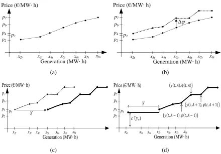
For hour 𝑡 and for each event 𝐴, the pairs (𝑦, 𝜓) are obtained, where 𝜓(𝑡, 𝐴) is the water
140
shadow price and 𝑦(𝑡, 𝐴) the hydro generation. Each event 𝐴 represents “one dot” in the short-run
141
marginal cost curve for the tth hour as shown in Fig. 1(d). The Fig. 1(d) is the final short-run marginal
142
cost curve of the hydro-wind coordination. The idea behind the primal and dual problem presented
143
in Eqs. (1) - (21) is the process of construction which starts with the short-run marginal cost curve of
144
the hydro generation [4] without the impact of wind power difference on the water shadow price [1]
145
as seen on Fig. 1(a). To include the impact of wind power difference on the water shadow price, the
146
wind power difference 𝑑, 𝑑+ and 𝑑− are implemented as discussed earlier. The resulting curve is
147
one in the Fig. 1(b) where the impact of wind power difference on the water shadow price, Δ𝜓, is
148
added to short-run marginal cost of hydro generation. The sign of Δ𝜓 depends on the sign of the
149
wind power difference i.e. the surplus of wind 𝑑+ means Δ𝜓 < 0 which reduces the water shadow
150
price while the shortage of wind 𝑑− means Δ𝜓 > 0 which increases the water shadow price in the
151
coordinated generation [1]. After accounting for the wind differences, the whole short-run marginal
152
cost curve should be horizontally shifted for forecasted wind generation, 𝑌, as shown in the Fig. 1(c).
153
This can be done since the effects of the wind generation on the generation range of hydro generation
154
in the previous curve (Fig. 1(b)). Finally, the short-run marginal cost 𝑐′(𝑦
𝑤) of wind generation 𝑦𝑤
156
should be added in a merit order way (based on ascending order of price). In the Fig. 1(c) the 𝑐′(𝑦 𝑤)
157
is lower than the water shadow price 𝜓 and is ranked before hydro generation, otherwise it would
158
be ranked last, or somewhere in the middle while shifting right part of the of the curve.
159
Price (€/MW∙ h)
Generation (MW∙ h)
x2t x3t x4t x5t x6t x7t x8tp7
p6
p4
p2
p3
Price (€/MW∙ h)
Generation (MW∙ h)
x2t x3t x4t x5t x6t x7t x8t
p7
p6
p4
p2
p3
∆ψ
(a)
(b)
Price
(€/MW∙ h)
Generation (MW∙ h)
x2t x3t x4t x5t x6t x7t x8t
p7
p6
p4
p2
p3
Y
Price
(€/MW∙ h)
Generation (MW∙ h)
x2t x3t x4t x5t x6t x7t x8t
p7
p6
p4
p2
p3
Y
c’
(
y
w)
(𝑦(𝑡,𝐴),𝜓(𝑡,𝐴))
(𝑦(𝑡,𝐴 −1),𝜓(𝑡,𝐴 −1))
(𝑦(𝑡,𝐴+ 1),𝜓(𝑡,𝐴+ 1))
(c)
(d)
Fig. 1 The example of construction of the joint short-run marginal cost curves
160
For the low market price events 𝐴 (and high opportunity cost) this approach would “force”
161
marginal cost curve to adjust itself (horizontally and vertically) until the water shadow price 𝜓 is
162
less or equal than market price 𝜋(𝑡, 𝐴) for some hour 𝑡, i.e. 𝜓(𝑡, 𝐴) ≤ 𝜋(𝑡, 𝐴): 𝑦(𝑡, 𝐴) > 0. Generally,
163
there is no generation when water shadow price is greater than market price4.
164
The implementation of the presented approach is simple, especially when having in mind that
165
the only needed equation for constructing marginal cost curves is the water shadow price 𝜓,
166
equation, Eq. (21). This equation can be used in the primal problems since the tools for modelling and
167
optimization usually enable readout of the optimal values of the dual variables, i.e. readout of the
168
shadow prices of each constraint. For calculating the water shadow price, the readout of tripe
169
consisting of shadow prices (𝜆, 𝜈𝑆𝑡, 𝜅𝑆𝑡) is needed.
170
3. Case study and Results
171
The primal and the dual problems are implemented with the GAMS Rev 239 modelling system
172
under the CPLEX solver. The study is done for the 5th December in 2016 on the case of wind farm
173
Vrataruša and hydropower system Vinodol, both located in Croatia. That specific week is considered
174
as the worst-case scenario from the standpoint of water scarcity and wind power differences. It is
175
assumed that wind farm Vrataruša and Vinodol hydropower system operate in hydro-wind
176
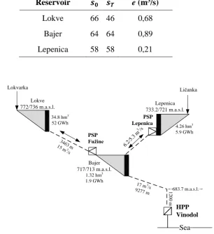
coordination and that they completely avoid balancing cost. The modelled Vinodol hydropower
177
system consists of: 3 reservoirs, 2 pumped-storage plants (PSP) and 1 hydropower plant (HP), with
178
details given in Table 1 and Fig. 2. The energy stock at the beginning/end of a day and the natural
179
water inflows are shown in Table 2. The difference between contracted and actual generated wind
180
power is given in Fig. 4. These input parameters are obtained from the real life middle-term operation
181
planning.
182
Table 1: HPS Vinodol facilities parameters.
183
Reservoir
k
St(GWh)
Power Plant
k
Tu/ n
Tu(m
3/s)
k
Tu/ n
Tu(MW)
Lokve 52 PSP Fužine 10/9 4.6/4.8
Bajer 1.9 HPP Vinodol 18.6 94.5
Lepenica 5.9 PSP Lepenica 6.2/5.3 1.14/1.25
Table 2: Energy stock in percent of maximum reservoir capacity 𝑘𝑆𝑡 at the beginning of and the end
184
of planning interval
185
Reservoir
𝒔
𝟎𝒔
𝑻e (m
3/s)
Lokve
66 46
0,68
Bajer
64 64
0,89
Lepenica
58 58
0,21
186
Lokvarka Ličanka
Lokve 772/736 m.a.s.l.
34.8 hm3 52 GWh
3463 m 15 m3
/s
PSP Fužine
Bajer 717/713 m.a.s.l.
1.32 hm3 1.9 GWh
Lepenica 733.2/721 m.a.s.l.
4.26 hm3 5.9 GWh
PSP Lepenica
6.2/ 5.3
m3/s
17 m3
/s
9277 m 12 683.7 m.a.s.l.
0
0
m
Sea
HPP Vinodol
187
Fig. 2 Model of the Vinodol hydropower system
188
The wind farm Vrataruša consists of 14 units, each with 3 MW of installed power. The total
189
installed power is 42 MW with minimum power output 1.1 MW. For the computational effectiveness,
190
only the hydro power plant Vinodol profit is maximized. There is no significant loss in accuracy since
191
the revenue of hydro power plant Vinodol participates with 95% in total system’s revenue. The ramp
192
rate limits of the hydro power plant Vinodol are: MSR (up) 255.15 (MW/min); MSR (down) 340.2
193
(MW/min). Therefore, there are no constraints on ramping capabilities in the model. The real
194
hydropower system Vinodol has conversion coefficient 𝜌 equal to 5.08 (MW/m3) and is used for
195
random number generator based on the statistical analyses of the Croatian nodal electricity prices of
197
the first week of December 2016 with the same probability of each event equal to 𝑃(𝐴) = 1 10, ∀𝑡 ∈
198
𝑇 ∀𝐴 ∈ ℱ𝑡. The CVaR percentile 𝛼 is 85%.
199
200
201
Fig. 4 The wind power difference (𝑑) for 5th December of 2016.
202
3.1 Results
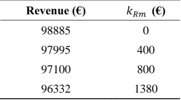
203
The results are shown in Table 3 and Fig. 5. The Table 3 shows the dependence of expected daily
204
revenue on the risk mitigation parameter 𝑘𝑅𝑚 used for hourly risk exposure reduction (it defines the
205
minimum expected return in the 1-α worst outcomes for each hour). The curves (Fig. 5) are for the
206
hourly risk exposure of 1380 € and 5 €/ MW∙h of short-run marginal costs of Vrataruša wind farm
207
generation.
208
Table 3 The expected daily revenue and associated risk exposure reduction 𝑘𝑅𝑚, ∀𝑡
209
Revenue (€)
𝑘
𝑅𝑚(€)
98885
0
97995
400
97100
800
96332
1380
210
-40 -35 -30 -25 -20 -15 -10 -5 0 5 10 15 20 25
1 2 3 4 5 6 7 8 9 10 11 12 13 14 15 16 17 18 19 20 21 22 23 24
d
(MW
∙h
)
Fig. 5 The short-run marginal costs curves for electricity generation of a Vinodol and Vrataruša
211
hydro-wind coordination.212
1.9
2.4
2.9
3.4
3.9
4.4
4.9
5.4
0
20
40
60
80
100
(€
/MW
∙h
)
(MW∙h)
1h
2h
3h
1.9
2.4
2.9
3.4
3.9
4.4
4.9
5.4
0
20
40
60
80
100
(€
/MW
∙h
)
(MW∙h)
4h
5h
6h
1.9
2.4
2.9
3.4
3.9
4.4
4.9
5.4
0
20
40
60
80
100 120
(€
/MW
∙h
)
(MW∙h)
7h
8h
9h
1.9
2.4
2.9
3.4
3.9
4.4
4.9
5.4
0
20
40
60
80
100 120
(€
/MW
∙h
)
(MW∙h)
10h
11h
12h
1.9
2.4
2.9
3.4
3.9
4.4
4.9
5.4
0
20
40
60
80 100 120 140
(€
/MW
∙h
)
(MW∙h)
13h
14h
15h
1.9
2.4
2.9
3.4
3.9
4.4
4.9
5.4
0
20
40
60
80 100 120 140
(€
/MW
∙h
)
(MW∙h)
16h
17h
18h
1.9
2.4
2.9
3.4
3.9
4.4
4.9
5.4
0
20
40
60
80
(€
/MW
∙h
)
(MW∙h)
19h
20h
21h
1.9
2.4
2.9
3.4
3.9
4.4
4.9
5.4
0
20
40
60
80
(€
/MW
∙h
)
(MW∙h)
3.2 Discussion
213
Risk mitigation and daily revenue. As parameter used for hourly risk exposure reduction 𝑘𝑅𝑚
214
increases from 0 € to 1380 €, the expected daily revenue decreased from 98 885 € to 96 332 € (Table 3).
215
Risk mitigation and the vertical shift of marginal cost curves. As parameter for hourly risk
216
exposure reduction 𝑘𝑅𝑚 increases from 0 € to 1380 €, the short-run marginal cost curves (Fig. 5) are
217
vertically shifted upwards from 1.9 €/MW∙h to approximately 2.5 €/MW∙h. This means that the hourly
218
risk exposure reduction has a certain cost that can be calculated from the marginal cost curves in Fig.
219
5. In average this cost is 2.5 €/MW∙h – 1.9 €/MW∙h = 0.6 €/MW∙h. Therefore 0.6 €/MW∙h is the price of
220
electricity which ensures owner with at least 1380 € in the worst-case scenario. Of course, this
221
insurance is at the expense of the daily revenue, which decreases.
222
Range of generation in marginal cost curves. The range of generation of Vrataruša-Vinodol
223
coordination is usually from 38 MW∙h to 58 MW∙h (Fig. 5). The one general conclusion can be drawn
224
regarding range of generation in joint marginal cost curves, that for low electricity prices (1h-3h and
225
22h- 24h) there is no desire to produce less than 38 MW∙h. It is obvious that in hours with higher
226
prices (13h-18h) coordination want to produce even more than 58 MW∙h and up to 80-90 MW∙h.
227
Prices in marginal cost curves. The short-run marginal cost curves are characterised by relatively
228
low (compared to market prices) cost which is a result of a low water shadow price. Perfectly inelastic
229
parts of the short-run marginal cost curves are obtained for the values 38 MW∙h and 58 MW∙h (Fig.
230
5).
231
4. Conclusion
232
The approach presented in this paper analyses the case of short-run hydro-wind coordination
233
which participates on the electricity market. This research contributes with the approach based on
234
duality method of convex programming for determining the joint short-run marginal cost curves for
235
an electricity generation of the hydro-wind coordination, which as a novelty combines risk mitigation
236
and the water shadow price. The proposed approach is easy to implement in various optimization
237
problems. Proposed method is suitable for investors with various risk preferences, from risk-averse
238
to risk-neutral or risk-seeking, since it enables risk mitigation. It has been shown that the perfectly
239
inelastic short-run marginal cost curves are appropriate for Vrataruša-Vinodol hydro wind
240
coordination which follows from the fact that the water shadow price was constant over the various
241
price events in particular hour. Therefore, it is justified to use simplified method for calculating water
242
shadow price which is constant over the planning period. It has been shown that the risk mitigation
243
has a cost and that this cost is easily quantified which is exemplified and discussed in the paper.
244
Acknowledgments: This research paper is made possible through the support from Department of Energy and
245
Power Systems of University of Zagreb Faculty of Electrical Engineering and Computing.
246
Author Contributions: Perica Ilak and Ivan Rajšl have contributed in developing the ideas and formulation of
247
the optimization problem. Josip Đaković and Marko Delimar have been involved in implementation of the
248
problem and analysis of the results. All the authors are involved in preparing the manuscript.
249
Conflicts of Interest: The authors declare no conflict of interest.
250
References
251
1. P. Ilak, I. Rajšl, S. Krajcar, and M. Delimar, "The impact of a wind variable generation on the hydro
252
generation water," Applied energy, vol. 154, pp. 197-208, April 2015.
253
2. A. Horsley and A. J. Wrobel, "Efficiency rents of storage plants in peak-load pricing, II: Hydroelectricty,"
254
London, 1999.
255
3. A Horsley and A J Wrobel, "Efficiency Rents of Storage Plants in Peak-Load Pricing, I: Pumped Storage,"
256
4. P. Ilak, S. Krajcar, I. Rajšl, and M. Delimar, "Pricing Energy and Ancillary Services in a Day-Ahead Market
258
for a Price-Taker Hydro Generating Company Using a Risk-Constrained Approach," Energies , vol. 7, no. 4,
259
5. R T Rockafellar, "Conjugate duality and optimization," Philadelphia (PA), 1974.
260
6. J. K. Kaldellis, M. Kapsali, and K. A. Kavadis, "Energy balance analysis of wind-based pumped hydro
261
storage systems in remote island electrical networks," Applied Energy, vol. 87, no. 8, pp. 2427-2437, 2010.
262
7. A. K. Varkani, A. Daraeepour, and H. A. Monsef, "A new self-scheduling strategy for integrated operation
263
of wind and pumped-storage power plants in power markets," Applied Energy, vol. 88, no. 12, pp.
5002-264
5012, 2011.
265
8. I. Rajšl, P. Ilak, M. Delimar, and S. Krajcar, "Dispatch Method for Independently Owned Hydropower
266
Plants in the Same River Flow," Energies, vol. 5, no. 9, pp. 3674-3690, 2012.
267
9. J. M. Angarita and J. G. Usaola, "Combining hydro-generation and wind energy: Biddings and operation
268
on electricity spot markets," Electric Power Systems Research, vol. 77, no. 5-6, pp. 393-400, April 2007.
269
10. J. L. Angarita, J. Usaola, and J. Martínez-Crespo, "Combined hydro-wind generation bids in a pool-based
270
electricity market," Electric Power Systems Research, vol. 79, no. 7, pp. 1038-1046, July 2009.
271
11. B. Vieira, A. Viana, M. Matos, and J. Pedro, "A multiple criteria utility-based approach for unit commitment
272
with wind power and pumped storage hydro," Electric Power Systems Research, vol. 131, pp. 244-254,
273
February 2016.
274
12. J. Duque, E. D. Castronuovo, , I. Sánchez, and J. Usaola, "Optimal operation of a pumped-storage hydro
275
plant that compensates the imbalances of a wind power producer," Electric Power Systems Research, vol. 81,
276
no. 9, pp. 1767-1777, September 2011.
277
13. R. T. Rockafellar and S. Uryasev, "Optimization of conditional value-at-risk," Journal of Risk, vol. 2, no. 3,
278
pp. 21-41, Sep 1998.
279
14. P. Artzner, F. Delbaen, J.M. Eber, and D. Heath, "Thinking coherently," Risk, vol. 10, pp. 68-91, 1997.
280
15. C. Acerbi, "Spectral measures of risk: A coherent representation of subjective risk aversion," J. Bank. Financ.,
281
vol. 26, pp. 1505-1518, 2002.
282
16. H. Follmer and A. Schied, "Convex and coherent risk measures," Berlin, 2008.
283
17. R.T. Rockafellar, "Coherent Approaches to Risk in Optimization Under Uncertanty," Tutor. Oper. Res. Inf.,
284
pp. 38-61, 2007.
285
18. R. T. Rockafellar and S. Uryasev, "Conditional Value-at-Risk for General Loss Distributions," Seattle, WA,
286
2001.
287
19. D. Perekhodtsev and L. Lave, "Efficient bidding for hydro power plants in markets for energy and ancillary
288
services," 2005.
289
20. T. C. Koopmans, "Water Storage Policy in a Simplified Hydroelectric System," in In Proceedings of the First
290
International Conference on Operational Research, Oxford, , 1957.
291
21. J. Warford and M. Munasinghe, "Electricity Pricing: Theory and Case Studies," Baltimore/London, 1982.
292
22. H. Zhang, F. Gao, J. Wu, K. Liu, and X. Liu, "Optimal Bidding Strategies for Wind Power Producers in the
293
Day-ahead Electricity Market," Energies, vol. 5, pp. 4804-4823, 2012
294
23. P. Ilak, S. Krajcar, I. Rajšl, and M. Delimar, "Profit Maximization of a Hydro Producer in a Day-Ahead
295
Energy Market and Ancillary Service Markets," in In Proceedings of the IEEE Region 8 Conference EuroCon,
296
Zagreb, 2013.
297