Compositional Distributional Semantics with Long Short Term Memory
Phong Le and Willem Zuidema
Institute for Logic, Language and Computation University of Amsterdam, the Netherlands
{p.le,zuidema}@uva.nl
Abstract
We are proposing an extension of the recur-sive neural network that makes use of a vari-ant of the long short-term memory architec-ture. The extension allows information low in parse trees to be stored in a memory reg-ister (the ‘memory cell’) and used much later higher up in the parse tree. This provides a so-lution to the vanishing gradient problem and allows the network to capture long range de-pendencies. Experimental results show that our composition outperformed the traditional neural-network composition on the Stanford Sentiment Treebank.
1 Introduction
Moving from lexical to compositional semantics in vector-based semantics requires answers to two dif-ficult questions: (i) what is the nature of the com-position functions (given that the lambda calculus for variable binding is no longer applicable), and (ii) how do we learn the parameters of those functions (if they have any) from data? A number of classes of functions have been proposed in answer to the first question, including simple linear functions like vec-tor addition (Mitchell and Lapata, 2009), non-linear functions like those defined by multi-layer neural networks (Socher et al., 2010), and vector matrix multiplication and tensor linear mapping (Baroni et al., 2013). The matrix and tensor-based functions have the advantage of allowing a relatively straight-forward comparison with formal semantics, but the fact that multi-layer neural networks with non-linear activation functions like sigmoid can approximate
any continuous function (Cybenko, 1989) already make them an attractive choice.
In trying to answer the second question, the ad-vantages of approaches based on neural network ar-chitectures, such as the recursive neural network (RNN) model (Socher et al., 2013b) and the con-volutional neural network model (Kalchbrenner et al., 2014), are even clearer. Models in this paradigm can take advantage of general learning procedures based on back-propagation, and with the rise of ‘deep learning’, of a variety of efficient algorithms and tricks to further improve training.
Since the first success of the RNN model (Socher et al., 2011b) in constituent parsing, two classes of extensions have been proposed. One class is to en-hance its compositionality by using tensor product (Socher et al., 2013b) or concatenating RNNs hor-izontally to make a deeper net (Irsoy and Cardie, 2014). The other is to extend its topology in order to fulfill a wider range of tasks, like Le and Zuidema (2014a) for dependency parsing and Paulus et al. (2014) for context-dependence sentiment analysis.
Our proposal in this paper is an extension of the RNN model to improve compositionality. Our mo-tivation is that, like training recurrent neural net-works, training RNNs on deep trees can suffer from the vanishing gradient problem (Hochreiter et al., 2001), i.e., that errors propagated back to the leaf nodes shrink exponentially. In addition, information sent from a leaf node to the root can be obscured if the path between them is long, thus leading to the problem how to capture long range dependen-cies. We therefore borrow the long short-term mem-ory (LSTM) architecture (Hochreiter and
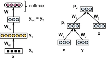
Figure 1: Multi-layer neural network (left) and Recursive neural network (right). Bias vectors are removed for the simplicity.
ber, 1997) from recurrent neural network research to tackle those two problems. The main idea is to allow information low in a parse tree to be stored in a memory cell and used much later higher up in the parse tree, by recursively adding up all mem-ory into memmem-ory cells in a bottom-up manner. In this way, errors propagated back through structure do not vanish. And information from leaf nodes is still (loosely) preserved and can be used directly at any higher nodes in the hierarchy. We then apply this composition to sentiment analysis. Experimen-tal results show that the new composition works bet-ter than the traditional neural-network-based com-position.
The outline of the rest of the paper is as fol-lows. We first, in Section 2, give a brief background on neural networks, including the multi-layer neural network, recursive neural network, recurrent neural network, and LSTM. We then propose the LSTM for recursive neural networks in Section 3, and its appli-cation to sentiment analysis in Section 4. Section 5 shows our experiments.
2 Background
2.1 Multi-layer Neural Network
In a multi-layer neural network (MLN), neurons are organized in layers (see Figure 1-left). A neuron in layeri receives signal from neurons in layeri−1
and transmits its output to neurons in layeri+ 1. 1 The computation is given by
yi =g Wi−1,iyi−1+bi
1This is a simplified definition. In practice, any layerj < i
[image:2.612.335.516.64.207.2]can connect to layeri.
Figure 2: Activation functions: sigmoid(x) = 1 1+e−x,
tanh(x) = e2x−1
e2x+1, softsign(x) = 1+x|x|.
where real vectoryi contains the activations of the neurons in layeri;Wi−1,i ∈R|yi|×|yi−1|is the ma-trix of weights of connections from layer i−1 to layer i; bi ∈ R|yi| is the vector of biases of the neurons in layeri; g is an activation function, e.g.
sigmoid,tanh, orsoftsign(see Figure 2).
For classification tasks, we put asoftmaxlayer on the top of the network, and compute the probability of assigning a classcto an inputxby
P r(c|x) =softmax(c) = P eu(c,ytop)
c0∈Ceu(c0,ytop) (1)
where u(c1,ytop), ..., u(c|C|,ytop)T = Wytop +
b; C is the set of all possible classes; W ∈
R|C|×|ytop|,b∈R|C|are a weight matrix and a bias
vector.
Training an MLN is to minimize an objective functionJ(θ)whereθis the parameter set (for clas-sification, J(θ) is often a negative log likelihood). Thanks to the back-propagation algorithm (Rumel-hart et al., 1988), the gradient∂J/∂θ is efficiently computed; the gradient descent method thus is used to minimizeJ.
2.2 Recursive Neural Network
with parse tree(p2 (p1x y)z)(Figure 1-right), and
that x,y,z ∈ Rd are the vectorial representations of the three wordsx,yandz, respectively. We use a neural network which consists of a weight matrix
W1 ∈ Rd×d for left children and a weight matrix
W2 ∈ Rd×dfor right children to compute the
vec-tor for a parent node in a bottom up manner. Thus, we computep1
p1 =g(W1x+W2y+b) (2)
wherebis a bias vector andgis an activation func-tion. Having computed p1, we can then move one
level up in the hierarchy and computep2:
p2=g(W1p1+W2z+b) (3)
This process is continued until we reach the root node.
Like training an MLN, training an RNN uses the gradient descent method to minimize an objective function J(θ). The gradient ∂J/∂θ is efficiently computed thanks to the back-propagation through structure algorithm (Goller and K¨uchler, 1996).
The RNN model and its extensions have been em-ployed successfully to solve a wide range of prob-lems: from parsing (constituent parsing (Socher et al., 2013a), dependency parsing (Le and Zuidema, 2014a)) to classification (e.g. sentiment analysis (Socher et al., 2013b; Irsoy and Cardie, 2014), para-phrase detection (Socher et al., 2011a), semantic role labelling (Le and Zuidema, 2014b)).
2.3 Recurrent Networks and Long Short-Term Memory
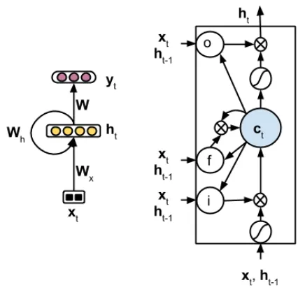
A neural network isrecurrent if it has at least one directed ring in its structure. In the natural lan-guage processing field, the simple recurrent neu-ral network (SRN) proposed by Elman (1990) (see Figure 3-left) and its extensions are used to tackle sequence-related problems, such as machine transla-tion (Sutskever et al., 2014) and language modelling (Mikolov et al., 2010).
In an SRN, an input xt is fed to the network at each time t. The hidden layer h, which has activation ht−1 right before xt comes in, plays a role as a memory store capturing the whole history
x0, ...,xt−1. Whenxtcomes in, the hidden layer updates its activation by
[image:3.612.319.532.54.263.2]ht=g Wxxt+Whht−1+b
Figure 3: Simple recurrent neural network (left) and long short-term memory (right). Bias vectors are removed for the simplicity.
whereWx ∈ R|h|×|xt|, Wh ∈ R|h|×|h|, b ∈ R|h| are weight matrices and a bias vector;gis an activa-tion.
This network model thus, in theory, can be used to estimate probabilities conditioning on long histo-ries. And computing gradients is efficient thanks to the back-propagation through time algorithm (Wer-bos, 1990). In practice, however, training recurrent neural networks with the gradient descent method is challenging because gradients∂Jt/∂hj(j ≤t,Jtis the objective function at timet) vanish quickly af-ter a few back-propagation steps (Hochreiaf-ter et al., 2001). In addition, it is difficult to capture long range dependencies, i.e. the output at timetdepends on some inputs that happened very long time ago. One solution for this, proposed by Hochreiter and Schmidhuber (1997) and enhanced by Gers (2001), islong short-term memory(LSTM).
Long Short-Term Memory The main idea of the LSTM architecture is to maintain a memory of
all inputs the hidden layer received over time, by
il-lustration in Graves (2012, Chapter 4)).
An LSTM cell (see Figure 3-right) consists of a memory cellc, an input gate i, a forget gate f, an output gate o. Computations occur in this cell are given below
it=σ Wxixt+Whiht−1+Wcict−1+bi
ft=σ Wxfxt+Whfht−1+Wcfct−1+bf
ct=ftct−1+
ittanh Wxcxt+Whcht−1+bc
ot=σ Wxoxt+Whoht−1+Wcoct+bo
ht=ottanh(ct)
where σ is the sigmoid function; it, ft, ot are the outputs (i.e. activations) of the corresponding gates;
ct is the state of the memory cell; denotes the element-wise multiplication operator; W’s andb’s are weight matrices and bias vectors.
Because the sigmoid function has the output range
(0,1)(see Figure 2), activations of those gates can be seen as normalized weights. Therefore, intu-itively, the network can learn to use the input gate to decide when to memorize information, and simi-larly learn to use the output gate to decide when to access that memory. The forget gate, finally, is to reset the memory.
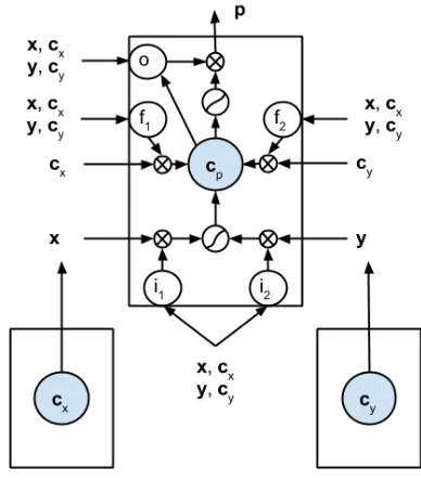
3 Long Short-Term Memory in RNNs In this section, we propose an extension of the LSTM for the RNN model (see Figure 4). A key feature of the RNN is to hierarchically combine in-formation from two children to compute the parent vector; the idea in this section is to extend the LSTM such that not only the output from each of the chil-dren is used, but also the contents of their memory cells. This way, the network has the option to store information when processing constituents low in the parse tree, and make it available later on when it is processing constituents high in the parse tree.
For the simplicity 2, we assume that the parent node p has two children aand b. The LSTM atp
thus has two input gatesi1, i2 and two forget gates f1, f2 for the two children. Computations occuring
in this LSTM are:
[image:4.612.329.523.65.287.2]2Extending our LSTM forn-ary trees is trivial.
Figure 4: Long short-term memory for recursive neural network.
i1 =σ Wi1x+Wi2y+Wci1cx+Wci2cy+bi
i2 =σ Wi1y+Wi2x+Wci1cy+Wci2cx+bi
f1 =σ Wf1x+Wf2y+Wcf1cx+Wcf2cy+bf
f2 =σ Wf1y+Wf2x+Wcf1cy +Wcf2cx+bf
cp =f1cx+f2cy+
g Wc1xi1+Wc2yi2+bc
o=σ Wo1x+Wo2y+Wcoc+bo
p=og(cp)
whereu andcu are the output and the state of the memory cell at nodeu;i1, i2,f1,f2,oare the
acti-vations of the corresponding gates;W’s andb’s are weight matrices and bias vectors; andgis an activa-tion funcactiva-tion.
Intuitively, the input gateij lets the LSTM at the parent node decide how important the output at the
j-th child is. If it is important, the input gate ij will have an activation close to 1. Moreover, the LSTM controls, using the forget gatefj, the degree to which information from the memory of thej-th child should be added to its memory.
com-plex sentence containing a main clause and a depen-dent clause it could be beneficial if only information about the main clause is passed on to higher lev-els. This can be achieved by having low values for the input gate and the forget gate for the child node that covers the dependent clause, and high values for the gates corresponding to the child node covering (a part of) the main clause. More interestingly, this LSTM can even allow a child to contribute to com-position by activating the corresponding input gate, but ignore the child’s memory by deactivating the corresponding forget gate. This happens when the information given by the child is temporarily impor-tant only.
4 LSTM-RNN model for Sentiment Analysis3
In this section, we introduce a model using the pro-posed LSTM for sentiment analysis. Our model, named LSTM-RNN, is an extension of the tional RNN model (see Section 2.2) where tradi-tional composition functiong’s in Equations 2- 3 are replaced by our proposed LSTM (see Figure 5). On top of the node covering a phrase/word, if its sen-timent class (e.g. positive, negative, or neutral) is available, we put a softmax layer (see Equation 1) to compute the probability of assigning a class to it.
The vector representations of words (i.e. word embeddings) can be initialized randomly, or pre-trained. The memory of any leaf node w, i.e. cw, is 0.
Similarly to Irsoy and Cardie (2014), we ‘untie’ leaf nodes and inner nodes: we use one weight ma-trix set for leaf nodes and another set for inner nodes. Hence, letdw anddrespectively be the dimensions of word embeddings (leaf nodes) and vector repre-sentations of phrases (inner nodes), all weight ma-trices from a leaf node to an inner node have size
d×dw, and all weight matrices from an inner node to another inner node have sized×d.
3The LSTM architecture was already applied to the
sentiment analysis task, for instance in the model proposed at http://deeplearning.net/tutorial/lstm. html. Independently from and concurrently with our work, Tai et al. (2015) and Zhu et al. (2015) have developed very similar models applying LTSM to RNNs.
Training Training this model is to minimize the following objective function, which is the cross-entropy over training sentence set D plus an L2-norm regularization term
J(θ) =−|D|1 X s∈D
X
p∈s
logP r(cp|p) +λ2||θ||2
whereθis the parameter set,cpis the sentiment class of phrasep,pis the vector representation at the node covering p, P r(cp|p) is computed by the softmax function, andλis the regularization parameter. Like training an RNN, we use the mini-batch gradient descent method to minimize J, where the gradient
∂J/∂θ is computed efficiently thanks to the back-propagation through structure (Goller and K¨uchler, 1996). We use the AdaGrad method (Duchi et al., 2011) to automatically update the learning rate for each parameter.
4.1 Complexity
We analyse the complexities of the RNN and LSTM-RNN models in the forward phase, i.e. computing vector representations for inner nodes and classifi-cation probabilities. The complexities in the back-ward phase, i.e. computing gradients∂J/∂θ, can be analysed similarly.
The complexities of the two models are domi-nated by the matrix-vector multiplications that are carried out. Since the number of sentiment classes is very small (5 or 2 in our experiments) compared todand dw, we only consider those matrix-vector multiplications which are for computing vector rep-resentations at the inner nodes.
For a sentence consisting of N words, assuming that its parse tree is binarized without any unary branch (as in the data set we use in our experiments), there areN−1inner nodes,Nlinks from leaf nodes to inner nodes, andN −2links from inner nodes to other inner nodes. The complexity of RNN in the forward phase is thus approximately
N ×d×dw+ (N−2)×d×d The complexity of LSTM-RNN is approximately
Figure 5: The RNN model (left) and LSTM-RNN model (right) for sentiment analysis.
In our experiments, this difference is not a prob-lem because training and evaluating the LSTM-RNN model is very fast: it took us, on a single core of a modern computer, about 10 minutes to train the model (d = 50, dw = 100) on 8544 sentences, and about 2 seconds to evaluate it on 2210 sentences.
5 Experiments 5.1 Dataset
We used the Stanford Sentiment Treebank4(Socher et al., 2013b) which consists of 5-way fine-grained sentiment labels (very negative, negative, neutral, positive, very positive) for 215,154 phrases of 11,855 sentences. The standard splitting is also given: 8544 sentences for training, 1101 for devel-opment, and 2210 for testing. The average sentence length is 19.1.
In addition, the treebank also supports binary sen-timent (positive, negative) classification by remov-ing neutral labels, leadremov-ing to: 6920 sentences for training, 872 for development, and 1821 for testing. The evaluation metric is the accuracy, given by
100×#correct
#total .
5.2 LSTM-RNN vs. RNN
Setting We initialized the word vectors by the 100-D GloVe5 word embeddings (Pennington et al., 2014), which were trained on a 6B-word cor-pus. The initial values for a weight matrix were uniformly sampled from the symmetric interval
−√1n,√1n where n is the number of total input
units.
4http://nlp.stanford.edu/sentiment/
treebank.html
5http://nlp.stanford.edu/projects/GloVe/
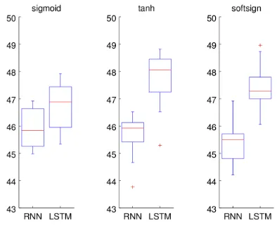
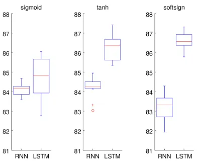
Figure 6: Boxplots of accuracies of 10 runs of RNN and LSTM-RNN on the test set in the fine-grained classifica-tion task. (LSTM stands for LSTM-RNN.)
For each model (RNN and LSTM-RNN), we tested three activation functions: softmax, tanh, and softsign, leading to six sub-models. Tuning those sub-models on the development set, we chose the dimensions of vector representations at inner nodes
d= 50, learning rate0.05, regularization parameter
λ= 10−3, and mini-batch-size 5.
On each task, we run each sub-model 10 times. Each time, we trained the sub-model in 20 epochs and selected the network achieving the highest ac-curacy on the development set.
Results Figure 6 and 7 show the statistics of the accuracies of the final networks on the test set in the fine-grained classification task and binary classifica-tion task, respectively.
[image:6.612.330.527.233.395.2]Figure 7: Boxplot of accuracies of 10 runs of RNN and LSTM-RNN on the test set in the binary classification task. (LSTM stands for LSTM-RNN.)
functions. With the sigmoid activation function, the difference is not so clear, but it seems that LSTM-RNN performed slightly better. Tanh-LSTM-LSTM-RNN and softsign-LSTM-RNN have the highest median accuracies (48.1 and 86.4) in the fine-grained clas-sification task and in the binary clasclas-sification task, respectively.
With the RNN model, it is surprising to see that the sigmoid function performed well, comparably with the other two functions in the fine-grained task, and even better than the softsign function in the bi-nary task, given that it was not often chosen in recent work. The softsign function, which was shown to work better than tanh for deep networks (Glorot and Bengio, 2010), however, did not yield improvements in this experiment.
With the LSTM-RNN model, the tanh function, in general, worked best whereas the sigmoid func-tion was the worst. This result agrees with the common choice for this activation function for the LSTM architecture in recurrent network research (Gers, 2001; Sutskever et al., 2014).
5.3 Compared against other Models
We compare LSTM-RNN (using tanh) in the pre-vious experiment against existing models: Naive Bayes with bag of bigram features (BiNB), Re-cursive neural tensor network (RNTN) (Socher et al., 2013b), Convolutional neural network (CNN) (Kim, 2014), Dynamic convolutional neural network
Model Fine-grained Binary
BiNB 41.9 83.1
RNTN 45.7 85.4
CNN 48.0 88.1
DCNN 48.5 86.8
PV 48.7 87.8
DRNN 49.8 86.6
with GloVe-100D
LSTM-RNN 48.0 86.2
with GloVe-300D
[image:7.612.91.288.65.225.2]LSTM-RNN 49.9 88.0
Table 1: Accuracies of the (tanh) LSTM-RNN compared with other models.
(DCNN) (Kalchbrenner et al., 2014), paragraph vec-tors (PV) (Le and Mikolov, 2014), and Deep RNN (DRNN) (Irsoy and Cardie, 2014).
Among them, BiNB is the only one that is not a neural net model. RNTN and DRNN are two ex-tensions of RNN. Whereas RNTN, which keeps the structure of the RNN, uses both matrix-vector multi-plication and tensor product for the composition pur-pose, DRNN makes the net deeper by concatenat-ing more than one RNNs horizontally. CNN, DCNN and PV do not rely on syntactic trees. CNN uses a convolutional layer and a max-pooling layer to han-dle sequences with different lengths. DCNN is hi-erarchical in the sense that it stacks more than one convolutional layers with k-max pooling layers in between. In PV, a sentence (or document) is rep-resented as an input vector to predict which words appear in it.
Table 1 (above the dashed line) shows the accura-cies of those models. The accuraaccura-cies of LSTM-RNN was taken from the network achieving the highest performance out of 10 runs on the development set. The accuracies of the other models are copied from the corresponding papers. LSTM-RNN clearly per-formed worse than DCNN, PV, DRNN in both tasks, and worse than CNN in the binary task.
5.4 Toward State-of-the-art with Better Word Embeddings
LSTM-RNN performed on par6 with their 1-layer-DRNN (d = 340) using dropout, which is to randomly remove some neurons during training. Dropout is a powerful technique to train neural networks, not only because it plays a role as a strong regulariza-tion method to prohibit neurons co-adapting, but it is also considered a technique to efficiently make an ensemble of a large number of shared weight neu-ral networks (Srivastava et al., 2014). Thanks to dropout, Irsoy and Cardie (2014) boosted the accu-racy of a 3-layer-DRNN withd = 200from 46.06 to 49.5 in the fine-grained task.
In the second experiment, we tried to boost the accuracy of the LSTM-RNN model. Inspired by Ir-soy and Cardie (2014), we tried using dropout and better word embeddings. Dropout, however, did not work with LSTM. The reason might be that dropout corrupted its memory, thus making train-ing more difficult. Better word embeddtrain-ings did pay off, however. We used 300-D GloVe word embed-dings trained on a 840B-word corpus. Testing on the development set, we chose the same values for the hyper-parameters as in the first experiment, except setting learning rate 0.01. We also run the model 10 times and selected the networks getting the high-est accuracies on the development set. Table 1 (be-low the dashed line) shows the results. Using the 300-D GloVe word embeddings was very helpful: LSTM-RNN performed on par with DRNN in the fine-grained task, and with CNN in the binary task. Therefore, taking into account both tasks, LSTM-RNN with the 300-D GloVe word embeddings out-performed all other models.
6 Discussion and Conclusion
We proposed a new composition method for the re-cursive neural network (RNN) model by extending the long short-term memory (LSTM) architecture which is widely used in recurrent neural network re-search.
6Irsoy and Cardie (2014) used the 300-D word2vec word
embeddings trained on a 100B-word corpus whereas we used the 100-D GloVe word embeddings trained on a 6B-word cor-pus. From the fact that they achieved the accuracy 46.1 with an RNN (d = 50) in the fine-grained task and 85.3 in the binary task, and our implementation of RNN (d = 50) per-formed worse (see Table 6 and 7), we conclude that the 100-D GloVe word embeddings are not more suitable than the 300-D word2vec word embeddings.
The question is why LSTM-RNN performed bet-ter than the traditional RNN. Here, based on the fact that the LSTM for RNNs should work very sim-ilarly to LSTM for recurrent neural networks, we borrow the argument given in Bengio et al. (2013, Section 3.2) to answer the question. Bengio explains that the LSTM behaves like low-pass filter “hence they can be used to focus certain units on differ-ent frequency regions of the data”. This suggests that the LSTM plays a role as a lossy compressor which is to keep global information by focusing on low frequency regions and remove noise by ignor-ing high frequency regions. So composition in this case could be seen as compression, like the recursive auto-encoder (RAE) (Socher et al., 2011a). Because pre-training an RNN as an RAE can boost the over-all performance (Socher et al., 2011a; Socher et al., 2011c), seeing LSTM as a compressor might explain why the LSTM-RNN worked better than RNN with-out pre-training.
Comparing LSTM-RNN against DRNN (Irsoy and Cardie, 2014) gives us a hint about how to im-prove our model. From the experimental results, LSTM-RNN without the 300-D GloVe word embed-dings performed worse than DRNN, while DRNN gained a significant improvement thanks to dropout. Finding a method like dropout that does not corrupt the LSTM memory might boost the overall perfor-mance significantly and will be a topic for our future work.
Acknowledgments
We thank three anonymous reviewers for helpful comments.
References
Marco Baroni, Raffaella Bernardi, and Roberto Zampar-elli. 2013. Frege in space: A program for composi-tional distribucomposi-tional semantics. In A. Zaenen, B. Web-ber, and M. Palmer, editors,Linguistic Issues in Lan-guage Technologies. CSLI Publications, Stanford, CA. Yoshua Bengio, Nicolas Boulanger-Lewandowski, and Razvan Pascanu. 2013. Advances in optimizing re-current networks. In Acoustics, Speech and Signal Processing (ICASSP), 2013 IEEE International Con-ference on, pages 8624–8628. IEEE.
superposi-tions of a sigmoidal function. Mathematics of control, signals and systems, 2(4):303–314.
John Duchi, Elad Hazan, and Yoram Singer. 2011. Adaptive subgradient methods for online learning and stochastic optimization. The Journal of Machine Learning Research, pages 2121–2159.
Jeffrey L. Elman. 1990. Finding structure in time. Cog-nitive science, 14(2):179–211.
Felix Gers. 2001. Long short-term memory in recur-rent neural networks. Unpublished PhD dissertation, ´Ecole Polytechnique F´ed´erale de Lausanne, Lausanne, Switzerland.
Xavier Glorot and Yoshua Bengio. 2010. Understand-ing the difficulty of trainUnderstand-ing deep feedforward neural networks. InInternational conference on artificial in-telligence and statistics, pages 249–256.
Christoph Goller and Andreas K¨uchler. 1996. Learning task-dependent distributed representations by back-propagation through structure. In International Con-ference on Neural Networks, pages 347–352. IEEE. Alex Graves. 2012. Supervised sequence labelling with
recurrent neural networks, volume 385. Springer. Sepp Hochreiter and J¨urgen Schmidhuber. 1997. Long
short-term memory. Neural computation, 9(8):1735– 1780.
S. Hochreiter, Y. Bengio, P. Frasconi, and J. Schmidhu-ber. 2001. Gradient flow in recurrent nets: the diffi-culty of learning long-term dependencies. In Kremer and Kolen, editors, A Field Guide to Dynamical Re-current Neural Networks. IEEE Press.
Ozan Irsoy and Claire Cardie. 2014. Deep recursive neural networks for compositionality in language. In
Advances in Neural Information Processing Systems, pages 2096–2104.
Nal Kalchbrenner, Edward Grefenstette, and Phil Blun-som. 2014. A convolutional neural network for mod-elling sentences. InProceedings of the 52nd Annual Meeting of the Association for Computational Linguis-tics (Volume 1: Long Papers), pages 655–665, Balti-more, Maryland, June. Association for Computational Linguistics.
Yoon Kim. 2014. Convolutional neural networks for sen-tence classification. InProceedings of the 2014 Con-ference on Empirical Methods in Natural Language Processing (EMNLP), pages 1746–1751, Doha, Qatar, October. Association for Computational Linguistics. Quoc Le and Tomas Mikolov. 2014. Distributed
repre-sentations of sentences and documents. In Proceed-ings of the 31st International Conference on Machine Learning (ICML-14), pages 1188–1196.
Phong Le and Willem Zuidema. 2014a. The inside-outside recursive neural network model for depen-dency parsing. InProceedings of the 2014 Conference
on Empirical Methods in Natural Language Process-ing. Association for Computational Linguistics. Phong Le and Willem Zuidema. 2014b. Inside-outside
semantics: A framework for neural models of semantic composition. InNIPS 2014 Workshop on Deep Learn-ing and Representation LearnLearn-ing.
Tomas Mikolov, Martin Karafi´at, Lukas Burget, Jan Cer-nock`y, and Sanjeev Khudanpur. 2010. Recurrent neural network based language model. In INTER-SPEECH, pages 1045–1048.
Jeff Mitchell and Mirella Lapata. 2009. Language mod-els based on semantic composition. InProceedings of the 2009 Conference on Empirical Methods in Natural Language Processing, pages 430–439.
Romain Paulus, Richard Socher, and Christopher D Man-ning. 2014. Global belief recursive neural networks. In Advances in Neural Information Processing Sys-tems, pages 2888–2896.
Jeffrey Pennington, Richard Socher, and Christopher D Manning. 2014. Glove: Global vectors for word rep-resentation. Proceedings of the Empiricial Methods in Natural Language Processing (EMNLP 2014), 12. David E Rumelhart, Geoffrey E Hinton, and Ronald J
Williams. 1988. Learning representations by back-propagating errors.Cognitive modeling, 5.
Richard Socher, Christopher D. Manning, and Andrew Y. Ng. 2010. Learning continuous phrase representa-tions and syntactic parsing with recursive neural net-works. InProceedings of the NIPS-2010 Deep Learn-ing and Unsupervised Feature LearnLearn-ing Workshop. Richard Socher, Eric H. Huang, Jeffrey Pennington,
An-drew Y. Ng, and Christopher D. Manning. 2011a. Dy-namic pooling and unfolding recursive autoencoders for paraphrase detection. Advances in Neural Infor-mation Processing Systems, 24:801–809.
Richard Socher, Cliff C. Lin, Andrew Y. Ng, and Christo-pher D. Manning. 2011b. Parsing natural scenes and natural language with recursive neural networks. In
Proceedings of the 26th International Conference on Machine Learning, volume 2.
Richard Socher, Jeffrey Pennington, Eric H Huang, An-drew Y Ng, and Christopher D Manning. 2011c. Semi-supervised recursive autoencoders for predicting sentiment distributions. InProceedings of the Confer-ence on Empirical Methods in Natural Language Pro-cessing, pages 151–161.
Richard Socher, John Bauer, Christopher D Manning, and Andrew Y Ng. 2013a. Parsing with compositional vector grammars. InProceedings of the 51st Annual Meeting of the Association for Computational Linguis-tics, pages 455–465.
Christopher Potts. 2013b. Recursive deep models for semantic compositionality over a sentiment treebank. InProceedings EMNLP.
Nitish Srivastava, Geoffrey Hinton, Alex Krizhevsky, Ilya Sutskever, and Ruslan Salakhutdinov. 2014. Dropout: A simple way to prevent neural networks from overfitting. The Journal of Machine Learning Research, 15(1):1929–1958.
Ilya Sutskever, Oriol Vinyals, and Quoc VV Le. 2014. Sequence to sequence learning with neural networks. In Advances in Neural Information Processing Sys-tems, pages 3104–3112.
Kai Sheng Tai, Richard Socher, and Christopher D Manning. 2015. Improved semantic representa-tions from tree-structured long short-term memory networks. arXiv preprint arXiv:1503.00075.
Paul J Werbos. 1990. Backpropagation through time: what it does and how to do it. Proceedings of the IEEE, 78(10):1550–1560.