University of New Hampshire
University of New Hampshire Scholars' Repository
School of Marine Science and Ocean Engineering
Institute for the Study of Earth, Oceans, and Space
(EOS)
12-1991
Remote estimation of the diffuse attenuation
coefficient in a moderately turbid estuary
Richard P. Stumpf
U.S.G.S.Jonathan Pennock
University of New Hampshire - Main Campus
Follow this and additional works at:
https://scholars.unh.edu/smsoe
Part of the
Hydrology Commons,
Natural Resources Management and Policy Commons, and the
Terrestrial and Aquatic Ecology Commons
This Article is brought to you for free and open access by the Institute for the Study of Earth, Oceans, and Space (EOS) at University of New Hampshire Scholars' Repository. It has been accepted for inclusion in School of Marine Science and Ocean Engineering by an authorized administrator of University of New Hampshire Scholars' Repository. For more information, please [email protected].
Recommended Citation
REMOTE SEN& ENVIRON. 38:183-191 (1991)
Remote Estimation of the Diffuse Attenuation
Coefficient in a Moderately Turbid Estuary
Richard P. Stumpf
U. S. Geological Survey, Center for Coastal Geology and Regional Marine Studies, St. Petersburg
Jonathan R. Pennock
University of Alabama, Marine Environmental Sciences Consortium, Dauphin Island
Solutions of the radiative transfer equation are used to derive relationships of water reflectance to the diffuse attenuation coej~cient (K) in moderately turbid water (K > 0.5 m-1). Data sets collected
from the NOAA AVHRR and in situ observations
from five different dates confirm the appropriate- ness of these relationships, in particular the logistic equation. Values of K calculated from the re- flectance data agree to within 60% of the observed values, although the reflectance derived using a more comprehensive aerosol correction is sensitive to chlorophyll concentrations greater than 50/zg
L - 1. Agreement between in situ and remote obser-
vations improves as the time interval between sam- ples is narrowed.
INTRODUCTION
Light availability is a critical regulator of estuarine primary production both for phytoplankton (Pen- nock and Sharp, 1986) and for seagrasses (Orth and Moore, 1983). As a result, both basic and management-related research efforts require in- formation on the availability of light in estuarine
Address correspondence to R. P. Stumpf, USGS Center for Coastal Geology and Marine Studies, 600 4th Street South, St. Petersburg, FL 33701.
Received 18 October 1990; revised 19 July 1991.
0034-4257 / 91 / $3.50
©Elsevier Science Publishing Co. lnc., 1991 655 Avenue of the Americas, New York, NY 10010
waters. Of particular interest is the measurement of the diffuse attenuation coefficient, which de- fines the presence of light versus depth, the depth of the euphotic zone, and ultimately the maximum depth of primary production.
Interest in water clarity and quality have lead to efforts to relate remote observations from satel- lite or airborne sensors to in situ light and optical measurements. Most studies in coastal and inland waters have compared remote observations to other types of optical data such as the Secchi disk depth and turbidity units (Khorram, 1985; Lathrop and Lillesand, 1986). In oceanic waters, Austin and Petzold (1981) found an empirical relationship between Coastal Zone Color Scanner (CZCS) observations and the diffuse attenuation coefficient for green light at 490 nm. However, because of limitations in the capability of the sensor and the atmospheric corrections, their re- sults are suitable only for waters having an attenu- ation coefficient of less than 0.5 m-1 and a pre- dominance of absorbing material, namely, case I and most case II waters.
Moderately turbid estuaries, those having diffuse attenuation coefficients from 0.5 m -1 to about 5 m-1, have optical characteristics deter- mined principally by scattering material, that is, suspended sediment, but with the interaction of multiple constituents, such as humic acids, iron
1 8 4 Stumpf and Pennock
compounds, and chlorophyll and related pig- ments. For these waters, which we shall refer to as case III (coastal) waters, following Jerlov's (1976) classification, there is a critical need for informa- tion on the attenuation coefficient.
Evaluating changes in the attenuation coeffi- cient in such waters is complicated by the strong spatial and temporal variability that occurs in these environments. Thus, studies often require frequent measurements. This would argue for the use of such data as that collected by the Advanced Very High Resolution Radiometer (AVHRR), which can provide imagery as often as twice daily during the summer.
Our recent demonstration of a physically and statistically strong relationship between water re- flectances observed from satellite and the total suspended sediment (or seston) in such waters in Delaware Bay on the Middle Atlantic Bight of the U.S. east coast (Stumpf and Pennock, 1989) leads us to investigate a relationship between water reflectance and the diffuse attenuation coefficient.
THEORY
Above-water irradiant reflectance in vertically ho- mogeneous, optically deep water can be ex- pressed in a form
R(X) = Y' bb(~,)
a(h) + bb(h)' (1)
where ~, is the wavelength or spectral band, bb is the backscatter coefficient, a is the absorption coefficient, and Y' (which will be assigned equal to 0.178) is a constant including surface refraction and reflection effects and a constant of proportion- ality (Gordon et al., 1975). In turbid (case III) water, Eq. (1) can be modified to
R(x) = r, b s(x)
s,(h) + ax(X) Ins'
(2)where b~s is the specific backscatter coefficient for the sediment (particulates) such that bbs=
b~,sns; s* is defined as b~s+as*, where as* is the specific absorption coefficient for the sediment
(as = as*n~), ax is the absorption coefficient for wa- ter, chlorophyll-related pigments, and dissolved pigments; and ns is the sediment concentration (Stumpf and Pennock, 1989).
The diffuse attenuation coefficient K for any wavelength or spectral band is defined as
I<- 1 at(z),
(3)dz
where E is the irradiance energy and z is the depth. Establishing a relationship between K and R depends on whether the water is absorption or scattering dominated. In case III waters, K is dependent primarily on the presence of sus- pended sediment (Biggs et al., 1983; Cloern, 1987), which has a strong backscattering compo- nent. We can then characterize K in terms of ns:
K = ks*ns + kx, (4)
where k* is the specific diffuse attenuation co- efficient for the suspended sediment or seston and kx is the diffuse attenuation coefficient for the other constituents (water, chlorophyll, etc.). If we assume that K varies only with ks (=k*ns) and that k~<<K, we can substitute (4) into (2) and obtain
b s(x)
R(x) = r, (5)
s*(),) + [ax(h)k*(h)] / K(h)'
Equation (5) can be modified to the logistic equa- tion
R ( x ) - (6)
1 +
where F* represents the sediment term (b~,s/s*)
and G*a represents the absorption term of (axk*/
s*). At long wavelengths where k~, the attenuation produced by the water, is not negligible, K' (= K - k w ) would formally replace K in Eq. (6). However, as kw at any one wavelength is constant, this modification is not of consequence, except when examining the physical significance of F* and G* in comparison to values derived from other measurements. This will be discussed later. We can also examine the role of sediment characteristics in Eq. (6). In Eq. (2), b~s and s* may vary, depending on the surface area, density, and scattering characteristics of the sediments. From Vande Hulst (1957), we can express these variables as
b *bs = bins/(pd), (7)
s* = s~n~/ (od), (8)
and
Estimation of Diffuse Attenuation in an Estuary 1 8 5
where subscript Q denotes the attenuation effi- ciency of the type of particle, p is the particle density, and d is the particle diameter. Clearly, variations in grain size and optical characteristics of the particles directly alter b~s, and also s* and k* in the same manner; therefore, some variation in R or K will be expected when comparing them with the sediment concentration [Eq. (2)]. Placing Eqs. (7)-(9) in Eq. (5) results in
R(x) = Y' b (x)
[s6(;~ ) + ax()~)k6(~)/K(~,)]' (10)
with the (pd) terms cancelling. Dividing through by s~) results in Eq. (6) again:
R(~,) - Y'F~(X)
1 + G*ao(~,)/K()~)' (11)
where the subscript Q simply denoted that F* and G*a are functions of only optical efficiency terms and not of particle size or density (F~)= F* and G*Q = G*).
As the particle size and density term (od) drops from the equation in producing Eq. (6), changes in sediment type should have a minor effect on the relationship between K and R. We should expect this result, as both R and K depend primarily on the surface area of the materials, whereas ns, which is a weight, depends on the volume and density of the material.
We can also examine a solution that does not involve an explicit assumption about the relation- ship between K and n~. Philpot (1987) presents a reflectance relationship based on a quasisingle scattering irradiance solution:
R ( x ) - , (12)
(KX) + Ku(X)
where Ku is the diffuse attenuation coefficient for upwelling light and B~s is the irradiant backscatter coefficient. Using Philpot's relationships,
Ku = aOu, (13)
B~ = K - aDd, (14)
where D is the distribution function for upwelling and downwelling light, we have
R(X) = K(),) - a(k)Dd(),) (15) K(~,) + a()~)Du(k)
and
R(~,) - 1 -fa(~,) / K(X) (16) 1 + ga(h) / K(~,)'
with fa = aDd and g~ = aDu. These equations also use K directly and not K ~. An equation having the form of Eq. (16) can be derived from Eq. (1) if we assume that K is a linear function of a and bb such that
K =cea +/3bb, (17)
where a and [3 are constants of proportionality (fa = o~a and ga =/3a - oLa).
In Eqs. (6) and (16), R will increase with K for fixed a. In ease I waters, however, R varies inversely with K (Morel and Prieur, 1977). Con- ceptually, the difference is straightforward: Where absorbing pigments are important such as most case I, and many case II, waters, increased pig- ments would increase K but absorb light other- wise available to leave the water column. Where particulates dominate, as in most ease III waters (and some case II waters), the increased scattering will increase both K and R. In ease III waters, pigments will still have the same effect as for ease I waters, namely, increase K and decrease R, but the absorption effect will be less important than that caused by scattering.
M E T H O D S
The processing for reflectance is described in more detail in Stumpf and Pennock (1989) and in Stumpf (1988). Briefly, the above-water reflec- tance from the satellite is found from
R(X) = ~rLw(X) / Ed(X), (18)
where the water-leaving radiance Lw is
Lw(h) = [L,(~,) - LA(h)] / TI(>,) (19)
the incident radiance on the water's surface, Ed, is approximated by
Ed(X) =E0(X) cos 00 T0(X), (20)
186 Stumpf and Pennock
(Stumpf, 1988). The aerosol component is cor- rected using the radiance over clear water, which has negligible refectance for red and near-IR light.
The total reflectance RT for the AVHRR is defined as
RT = ~[Lw(1) + Lw(2)] (21) Ea(1) + E,~(2) '
where 1 denotes AVHRR Band 1 (red, 580-680 nm) and 2 denotes AVHRR Band 2 (near-infrared, 720-1000 nm). It was previously shown that R~ reduces the effect of chlorophyll-a absorption of red light, while increasing sensitivity over use of the near-infrared band alone (Stumpf and Pen- nock, 1989). However, use of RT with the AVHRR requires assumption of an areally uniform atmo- sphere, which is not a frequent occurrence. To correct for spatial variability, we find a reflectance
Ro corrected for aerosol variations at each pixel
Ro = R(1) - AR(2). (22)
Assigning A = 1.0 provides an effective correction for such aerosols as cirrus clouds and for glint. [Other values for A could be found by determining the values of R(1) and R(2) in clearwater, that is, where Ro = 0.] Ro is generally proportional to R(1); hence it may be affected by variations in pigments that absorb red light.
The use of the AVHRR has certain advantages in estuarine waters. The near-IR band lies outside the range of effect of most pigments, simplifying some of the absorption problems. The dominant nonchlorophyll pigments, such as the humic acids, iron, and carotenoids, have the greatest effect on shorter wavelengths, especially blue and green; therefore, they will have a greatly reduced [but not always negligible (Witte et al., 1982)] effect on red light. Finally, estuarine case III waters often contain these materials that strongly absorb shorter wavelengths, resulting in the wavelength of maximum light penetration in the water at about 600 nm. This wavelength lies within the bounds of the AVHRR Band 1.
Satellite Data Processing
The AVHRR data sets were obtained as level 1B format digital data (Kidwell, 1986). The scenes were processed to a Mercator projection with a pixel size of 1.18 km at 39°N. To reduce naviga- tion errors in the data, the images were shifted
linearly to match the shoreline to within 1 pixel of a digitally overlain database shoreline. Five images from spring of 1987 were used: NOAA-9 from 5 and 6 March, 22 March, and 28 May and NOAA-10 for 30 April.
Valid comparisons of points in the image data to the shipboard stations require relocation of the sampling position to account for tidal motion, as described in Stumpf and Pennock (1989). The median value of the 3 x 3 block of pixels around each of these relocated points (based on predicted tidal currents) was used for analysis against the shipboard observation.
In situ Methods
In situ observations were made on four cruises (SCENIC-7, -8, -10, -11), corresponding to the dates of the AVHRR imagery. Diffuse attenuation was determined from measurements made with a Biospherical Instruments QSR-100 underwater irradiance meter. This meter provides integrated observations of the photosynthetically active radi- ation from 400 nm to 700 nm. Measurements were made at 0.25-0.5 m intervals, with deck observations made to assure constancy of the inci- dent light during the measurement period. Based on the solution to (3), namely Beer's law, K was found from linear regression of In [E(z)/E(zo)] against z, where Zo is the uppermost depth of measurement. In all cases evaluated, r 2 was greater than 0.97.
Water samples were taken from Niskin bottles at 0.5-1.0 m below the surface. Profiles with transmissometer ,and the irradiance measure- ments showed no variation in the optical charac- teristics of the water in the upper few meters. Suspended sediment concentrations were deter- mined gravimetrically following filtration onto preweighed 1.0 tzm Nucleopore filters and vac- uum desiccation. Chlorophyll-a was determined fluorometrically following the method of Strick- land and Parsons (1972), using the acid correction for phaeophytin as described by Lorenzen (1967). These and other field measurements are de- scribed in Pennock (1985).
RESULTS
Estimation of Diffuse Attenuation in an Estuary 18 7
5 . 0 -
4 . 0
V 3 . 0 Z 0
I - I
I - <~ 2 . o
~) Z LU F- <~
1 . 0
13
5
13 [ ]
0 . 0 ~
0 10 2 0
13
[ ] O [ ] [ ]
3 0 4 0
S E S T O N ( M G / L ) [ ]
13
K - 0 . 0 7 4 n s + 0 . 6 t
R - 0 . 9 6
DELAHARE BAY MAR-HAY 1 9 8 7
5 0 6 0
Figure 1. K vs. seston (or total suspended sedi- ments).
lower Delaware Bay (Fig. 1). Although the slope of this relationship is similar to that found in other studies in lower Delaware Bay (Pennock, 1985), the relation could be affected by changes in the size and optical characteristics of the sediment. For example, a different slope applies in the Dela- ware River turbidity maximum, although the lin- ear relationship still applies (Biggs et al., 1983).
Equation (6) accurately represents the rela-
tionship between RT and K (Fig. 2). When applied to data pairs collected within 3.5 h, over 95% of the variance in the data can be explained by the relationship with a standard error of 0.003 (reflectance units) about the equation solution. Similarly, Eq. (16) also represents the data, show- ing the same shape as Eq, (6) over the range. Slightly larger errors for points collected further apart in time is expected as a result of spatial
o.o4o
T
O. 0 3 0
F- r r W Z <~
I-. o . 0 2 0
W _1 LL W r r
0 . 0 t 0
0 . 0 0 0
0 . 5
4
• < 3 . 5 HOURS / / 0 SAME DAY ~ • / /
* DZFFERENT DAY / /
D
.
[ ] m J
° °
m /
[]
DELAWARE BAY MAR-MAY 1 9 8 7
I 1 I I I I I I I
1 . 0 5 . 0
188 Stumpf and Pennock
0 . 0 3 0
rl- o . 0 2 0 LU
Z
<~ I"- U LLI _J LL LLI IT' O . O t C
A > 5 0 U G / L C H L - A 0 3 0 - 5 0 UG/L [ ] < 3 0 U S / L
F I L L E D < 3 . 5 H
- - E Q . 6
- - E Q . 16
O []
[]
[ ]
J [] []
Q
0 . 0 0 O t ' I I l 1 I " " I 0 . 5 ' t . 0
0
[ ] A • ,
A T T E N U A T I O N K (I/M)
[ ]
A
AVHRR DELAWARE BAY MAR-MAY 1 9 8 7
I I
5 . 0
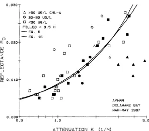
Figure 3. Ro v s . K .
variability and both the tidal and wind-driven excursion (Stumpf and Pennock, 1989). These results suggest that in situ and remote observa- tions should be taken within 3 h of each other for valid calibration, even when applying a correction for tidal motion. Without corrections for water movement, lags of less than 1-2 h are preferable. A plot of RD vs. K shows a strong relationship of the form of Eqs. (6) and (16) provided that the chlorophyll concentration remains below 50 # g / L (Fig. 3). The absorption produced by high chloro- phyll concentrations decreases Band 1 reflec- tance, thereby decreasing RD relative to K. Points having chlorophyll concentrations of 30-50 #g L-1 tend to lie at or below the curve. Of the five points in this class that lie well above the curve, four consist of satellite and in situ observtions taken a day apart; hence less significance should
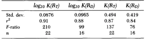
be ascribed to these points. Table 1 shows the coefficients from Eq. (6) for R~ and RD.
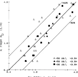
As variability in K tends to increase in propor- tion to the value of K, the log transform appropri- ately represents the distribution of the two sets of K (this fact is confirmed by the higher r 2 for the log regression than for the linear regression) (Table 2). When comparing K as estimated from R~ to the in situ observations, the results corre- spond to within 55 % at the 95 % confidence level (Fig. 4). Similarly, using RD, the estimated and observed values of K have a 95% confidence interval (C.I.) of'60% when the chlorophyll con- centration is < 50 #g L-1 (Fig. 5).
The scatter in the relationship between ob- served and calculated K closely matches that found for seston in Stumpf and Pennock (1989). As they described, the discrepancy between ob-
Table 1. S t a t i s t i c s f o r E q . (6)
RD RD RT vs. K '
RT < 30 #g L - I < 50 #g L -1 Kw= 0.5 <3.5 h <3.5 h <3.5 h <3.5 h
F* 0 . 5 5 ± 0 . 2 3 0 . 4 9 ± 0 . 2 6 0 . 6 3 ± 0.41 0 . 3 0 ± 0 . 0 6 G* 9.1 ± 5 . 1 8 . 2 ± 5 . 8 1 1 . 6 ± 9 . 1 2 . 8 ± 0 . 9
Std. dev. 0 . 0 0 3 7 9 0 . 0 0 2 8 8 0 . 0 0 2 7 9 0 . 0 0 3 7 2
n 2 2 12 16 2 2
Estimation of Diffuse Attenuation in an Estuary 189
Z
rr
0 r r LL
4.0
~" i.O
[] D r " / / / / /
Z /
/ / / /
n
, / /
D / " + 5 5 =
[] ,/" •
/ i i / / • .
[] /El'~ • • • / t/ / /
/ /"
/
/ / / S/ / /
• f /
•
///
]
• , //
.?
> 5 0 U G / L > 3 . 5 H • >50 U 6 / L < 3 . 5 H D <50 U 6 / L >~.SH
• <50 U 6 / L < ~ . S H
0 . 4 ~ I I I
0 . 4 1 . 0 4 . 0
I N S Z T U K ( I I M )
I i
Figure 4. K derived from Rr vs. observed K; dot- ted line shows the 95% confidence interval of the regression.
served and calculated values results from several
factors: errors in the determination of both K (in situ) and R; unknown movements or mixing in the water between overpass and sample; and the difference in the scales of the observations. It is not unexpected that m o v e m e n t o f the water
causes significant discrepancies, even with the correction for tidal motion. Samples taken more than 3.5 h apart show differences of > 60%, and those taken on the preceding day can differ by a factor of 2. As other factors, such as wind and high river flow, can produce water movement that
4 . 0 T
!
i
4-
rn r r :E 0 rT- i . O " h x.."
0 . 4 ¥ 1 0 . 4
pJ~ pJ~ ppJS
/// • //"
/ / / ~ / / /
~ / I A • / / /
/ / ~ / /
/// • & //
//" • ~ / /
• .//
/ / " • < 3 0 UG/L < 3 . 5 H
I / ] I 1 1 I 1 I
1 . 0 4 . 0
I N S I T U K ( I / M )
Figure 5. K derived from Ro vs. observed K for
1 9 0 Stumpf and Pennock
Table 2. K Estimated from Reflectance vs. K Observed
loglo K(RT) loglo K(RD) K ( R T ) K(RD)
Std. dev. 0.0876 0.0965 0.494 0.419
r 2 0.91 0.88 0.87 0.84
F-ratio 210 99 137 76
n 22 16 22 16
cannot be estimated, smaller differences should be obtainable by taking samples within 1-2 h of an overpass.
The difference in scale, however, will remain a source of discrepancy. Reflectance is an average of a 1.2 km 2 area, but K is obtained from measure- ments in a much smaller parcel of water. Even given ideal atmospheric conditions and perfect measurement and navigation, the difference in sampling area will always produce some discrep- ancy. Stumpf and Pennock (1989) estimated dis- crepancies as large as 30 % for seston, a significant portion of the total difference. In areas of strong fronts, greater differences may occur.
DISCUSSION
Chlorophyll alters the absorption coefficient; therefore, we can expect additional chlorophyll to increase G*a in Eq. (6), which in turn causes R to decrease. This effect is strongest for Ro because this reflectance value behaves like Band 1, which includes chlorophyll absorption bands. In this data set, if G* is increased to 22 m-1, the curve will pass through the group of points in Figure 3 having chlorophyll concentrations greater than 50 /xg L -1.
The coefficients derived by substituting K' for K in (6) should be physically meaningful. The results (column 4 of Table 1) are reasonable. As
- b * * +
F* is equivalent to b*bs/s* (= bs/[bbs a*]), it must be less than 1 (it was found to be 0.30). G* represents the absorption term of (axk*/s*).
This should be somewhat greater than the absorp- tion coefficient of water as ax is somewhat greater than aw and k * / s * is slightly greater than one. For the AVHRR, aw is about 0.3 m-1 for Band 1 and greater than 2 m-1 for Band 2; hence the observed value of 2.8 m - 1 is appropriate.
In Eq. (16), the values of the coefficients cannot be meaningfully evaluated. Similar curves can be obtained with substantially different val-
ues, particularly for f~. The similarity between the graphs of Eqs. (6) and (16) is not surprising be- cause (6) can be treated as an approximation to (16) for large values of K. When K becomes much larger than fa, the numerator in (16) varies little relative to the denominator and can therefore be treated as a constant resulting in an equation of the form of (6).
The relationship between K and ns (Fig. 1) suggests relatively little variation in the sediment characteristics during the sampling period; thus we could not evaluate the hypothesis that factors such as particle size and density will have a negli- gible effect on the relation of reflectance and diffuse attenuation [Eqs. (10) and (11)]. If this proves to be the case, then the coefficients in Eq. (6) may apply to a variety of estuaries, particularly when the chlorophyll content remains below 50 #g L -1.
CONCLUSIONS
Equations (6) and (16) provide appropriate repre- sentations of the relationship between remotely observed reflectance and observations of the diffuse attenuation coefficient. The coefficients pre- sented here for (6) have applicability to NOAA-9 and NOAA-10 data collected in 1987. The stability of the Band 1 and 2 responses is not quite clear (Abel et al., 1988); if the calibration from digital counts to reflectance varies over time, and cannot be accurately determined, some recalculation of the Eq. (6) coefficients will be necessary for different times.
Further comparison of data from different areas can be used to evaluate the variability in the coefficients of (6). By comparing reflectance or attenuation coefficients with sediment concen- tration, we could identify areas having sediments with optically significant differences. Thus, these areas could be compared for their relationships between R and K. Equation (6) also has the advan- tage of being a standard logistic equation and so allows multiple ways of deriving regression solutions.
Estimation of Diffuse Attenuation in an Estuary 191
REFERENCES
Abel, P., Smith, G. R., and Levin, R. H. (1988), Results from aircraft measurements over White Sands, New Mexico, to calibrate the visible channels of spacecraft instruments, SPIE, Ocean Optics IX, Orlando, Florida, April 1988, No. 924, 208-214.
Austin, R. W., and Petzold, T. J. (1981), The determination of the diffuse attenuation coefficient of sea water using the coastal zone color scanner, in Oceanography from Space, (J. F. R. Gower, Ed.), Plenum, New York, pp. 239- 256.
Biggs, R. B., Sharp, J. H., Church, T. M., and Tramantano, J. M. (1983), Optical properties, suspended sediments, and chemistry associated with the turbidity maxima of the Delaware estuary, J. Can. Fisheries Aquatic Sci. 40 (Suppl. 1):172-179.
Cloern, J. E. (1987), Turbidity as a control of phytoplankton biomass and productivity in estuaries, Continental Shelf Res. 7:1367-1381.
Gordon, H. R., Brown, O. B., and Jacobs, M. M. (1975), Computed relationships between the inherent and appar- ent optical properties of a fiat homogeneous ocean, Appl. Opt. 14:417-427.
Jerlov, N. G. (1976), Optical Oceanography, Elsevier, New York.
Khorram, S. (1985), Development of water quality models applicable throughout the entire San Francisco Bay and Delta, Photogramm. Eng. Remote Sens. 51(1):53-62. Kidwell, K. B. (1986), NOAA Polar Orbiter Data (TIROS-N,
NOAA-6, NOAA-7, NOAA-8, NOAA-9, NOAA-IO) Users Guide, revised January 1988, National Oceanographic and Atmospheric Admin., National Environmental Satellite Data and Information Service, Washington, DC. Lathrop, R. G., and Lillesand, T. M. (1986), Use of Thematic
mapper data to assess water quality in Green Bay and central Lake Michigan, Photogramm. Eng. Remote Sens. 52:671-680.
Lorenzen, C. J. (1967), Determination of chlorophyll and pheo- phytin: spectrophotometric equation, Limnol. Oceanogr. 12:343-346.
Morel, A., and Prieur, L. (1977), Analysis of variations in ocean color, Limnol. Oceanogr. 22(4):709-722.
Orth, R. J., and Moore, K. A. (1983), Chesapeake Bay: an unprecedented decline in submerged aquatic vegetation, Science 222:51-53.
Pennock, J. R. (1985), Chlorophyll distributions in the Dela- ware Estuary: regulation by light-limitation, Estuarine, Coastal, Shelf Sci. 21:711-725.
Pennock, J. R., and Sharp, J. H. (1986), Phytoplankton pro- duction in the Delaware estuary: temporal and spatial variability, Mar. Ecol. Prog. Ser. 34:143-155.
Philpot, W. D. (1987), Radiative transfer in stratified waters: a single-scattering approximation for irradiance, Appl. Opt. 26(19):4123-4132.
Strickland J. D. H, and Parsons T. R. (1972), A Practical Handbook of Seawater Analysis, Bulletin Fisheries Re- search Board of Canada #167, Ottawa, 310 pp.
Stumpf, R. P. (1988), Remote detection of suspended sedi- ment concentrations in estuaries using atmospheric and compositional corrections to AVHRR data, in Proc. 21st Int. Symposium on Remote Sensing of Environment, 26-30 October 1987, ERIM, Ann Arbor, MI, pp. 205-222.
Stumpf, R. P., and Pennock, J. R. (1989), Calibration of a general optical equation for remote sensing of suspended sediments in a moderately turbid estuary, J. Geophys. Res. Oceans 94(C10):14,363-14,371.
Vande Hulst, H. C. (1957), Light Scattering by Small Particles, Wiley, New York.