Manuscript received November 18, 2014; revised March 12, 2015; revised May 21, 2015, accepted June 25, 2015. Paper 2014-IPCC-0846.R2, presented at the 2014 IEEE Energy Conversion Congress and Exposition, Pittsburgh, PA, September 14–18, and approved for publication in the IEEE TRANSACTIONS ON INDUSTRY APPLICATIONS by the IEEE-IAS Industrial Power Converter Committee of the IEEE Industry Applications
Society.
Grid Parameter estimation using Model Predictive
Direct Power Control
Bilal Arif*, Luca Tarisciotti, Pericle Zanchetta, Jon Clare, Marco Degano
Department of Electrical and Electronics Engineering,The University Of Nottingham, Nottingham, UK *[email protected]
Abstract – This paper presents a novel Finite Control Set Model Predictive Control (FS-MPC) approach for grid-connected converters. The control performance of such converters may get largely affected by variations in the supply impedance, especially for systems with low Short Circuit Ratio (SCR) values. A novel idea for estimating the supply impedance variation, and hence the grid voltage, using an algorithm embedded in the MPC is presented in this paper. The estimation approach is based on the difference in grid voltage magnitudes at two consecutive sampling instants, calculated on the basis of supply currents and converter voltages directly within the MPC algorithm, achieving a fast estimation and integration between the controller and the impedance estimator. The proposed method has been verified, using simulation and experiments, on a 3-phase 2-level converter.
I. INTRODUCTION
The extended use of Renewable and Distributed Generation (DG) systems in the past decade is widely contributing to modify the old concept of electrical distribution network towards an “active” model where power can flow in any direction [1]. This has demanded an improvement in power electronics systems and control in order to implement systems grid interface, effective and intelligent power flow control and to avoid grid instability [2]. The application of power electronics converters and in particular grid connected technology or Active Front End (AFE) has become a key enabling technology in all renewable and distributed generation systems like, for example, photovoltaic and wind power generation systems [1], [3]. AFE can be also used as active filters where they are connected in parallel or series to a non-linear load and offer reduction in harmonics production [4], [5]. In these scenarios the converter control is a key element to achieve optimal generation systems grid interface, the required power flow and to avoid grid instability [6]. In contrast with traditional control techniques applied to AFE, such as Voltage Oriented Control (VOC) [7] and Direct Power Control (DPC) [8], Finite Control Set Model Predictive Control (MPC) has been recently proved to represent a promising solution to control of power electronics converters. In fact, it provides several advantages including better dynamic response, flexible control action and digital implementation [9], [10], [11]. In particular, several MPC strategies have been proposed in
literature for grid connected converters; some solutions implement just a current control [12], [13], [14], while others investigate a more complete direct power control [5], [15], [16]. In [5],[15], the authors propose a Model Predictive Direct Power Control (MP-DPC) approach; it allows to eliminate the external PI based DC-link voltage controller, hence avoiding windup issues or linearization of the system for proper tuning of the PI controllers. However, as any model based control technique, MP-DPC is sensitive to model parameter variations. In Figure 1, while the converter inductance, Lc, and its parasitic resistance, r, are usually known, the grid parameters (usually inductance dominant,
Ls), are unknown and can have highly varying values depending on the grid load conditions. Since MP-DPC is based on the knowledge of model parameters, any small variations in these parameters will disturb performance and stability of the control system.
consecutive sampling instants, [21], [24], and it is integrated within the MPC algorithm. The supply resistance is not considered in this work, since its effect can be considered negligible with respect to the supply inductance which heavily affects the magnitude and phase of the grid voltage, thus reducing the performance of the MPC. However, it is always possible to expand the proposed estimation method to include the supply resistance estimation.
The combination of a finite set MP-DPC and the proposed estimation algorithm results in a high-bandwidth control robust to supply impedance variations without increasing excessively the complexity of the control system.
II. MODEL PREDICTIVE -DPCAPPROACH
[image:2.595.310.544.148.226.2]The equivalent circuit in αβ reference frame calculated using [25], of the AC side of the AFE system in Figure 1 is shown in Figure 2.
Figure 1. Grid-connected active front-end rectifier
Figure 2. Equivalent AFE model in α and β reference frames
The continuous-time representation for this equivalent circuit is given in (1), while the continuous time model for the system DC side is given in (2).
∙ 1 ∙ 1
! " ∙ ! 2
In (1)-(2) vgrid, vc and Vdc are, respectively, grid, converter and DC-link voltage; is and idc are supply and converter DC current, the total inductance L, is the sum of converter filter inductance LC and supply inductance LS, r is the converter input filter resistance, R is the load resistance and C is the dc-link capacitance. In order to obtain the desired prediction of the supply current, the current derivative is approximated using the Euler forward method as mentioned in [11]. Since
the MPC works in discrete-time, the following equations represent the discrete-time model of the continuous-time system given in (1) and (2):
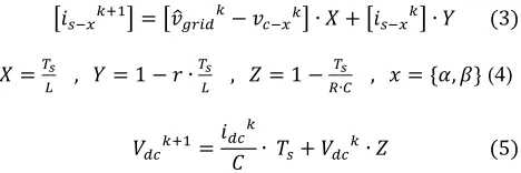
$%& ' $ $ ∙ ( ) $ ∙ * 3
( ,
-. , * 1 ∙ ,
-. , 0 1 ,
-1∙2 , 3 45, 67 (4)
$%& $
! ∙ 8 ) $∙ 0 5
The predictions are made for a future sampling instant
k+1, using the information provided at the present instant k.
In the practical implementation, due to the calculation time required by the digital control system, a delay of one sampling instant is taken into consideration by making predictions at instant k+2. Hence the model becomes:
$%: ' $%& $%& ∙ ( ) $%& ∙ * 6
< = $%:
$%&
! ∙ 8 ) $%&∙ 0 7
where, vck+1 and idck+1 are calculated using the optimized switching signals from the predictive controller at the previous sample interval k. Having the supply current predictions at k+2, the active and reactive powers, predictions respectively at this sampling instant are
?< = $%: 32 @' A$%:∙ A$%:) ' B$%:∙ B$%:C 8
E< = $%: 32 ' B$%:∙ A$%: ' A$%:∙ B$%: 9
Equations (7)-(9) are calculated for every possible converter states; between all of them, the state to apply is selected using a user defined cost function, which represents DC-Link voltage, Active and Reactive power errors. The cost function and the required references calculation are described in the following subsections.
A. DC-link voltage reference
The method proposed in [5] and [15] was adopted to obtain suitable references for the active power and the dc-link voltage. The reference dc-dc-link voltage is calculated using (10) where N* is the reference prediction horizon. A suitable selection of N* results in a better dynamic response of the dc-link voltage.
=G$%& $)H1∗@ =G$ $C 10
[image:2.595.63.275.301.522.2]B. Power reference
The reactive power reference Qrefk+2 is kept to 0 VAR to obtain unity power factor operation. Thus, without using any Phase-Locked-Loop (PLL), as is the case in current control where the grid phase angle estimation is necessary for current reference generation, the supply voltage and current are synchronized by maintaining a close to unity power factor by directly controlling active and reactive powers. Moreover, under low SCR scenarios, re-tuning of PLL algorithmsmay have computational constraints, adding more complexities to the control structure. Therefore, assuming unity power factor, the active power reference is calculated using the system power balance equation [15] as shown in (11) where, Ps is the supply active power, Pr is the power loss on the input filter resistance and Pload is the active power across the capacitor and resistor at the DC side.
? ? ) ?KLM 11
For a balanced and undistorted 3-phase system with a unity power factor, it can be assumed that
? 32 ' $%& $%& 12
? 32 @ $%& C: 13
where $%& and ' $%&are the predicted supply current and estimated grid voltage obtained from (3) and (36), respectively. Therefore, (11) can be expressed in a discretized form in terms of grid voltage and supply current, with regards to Figure 1, as shown in (14).
$%&: ' $%& $%&)2?KLM $%&
3 0 14
Solving (14) for isk+1 and multiplying by ' $%&, the active supply power reference is hence obtained in (17), where Pload is the load power and idck+1 is the rectified current defined, respectively, by (15) and (16).
?KLM $%& $%&∙ =G$%& 15
$%& ! ∙ =G$%& $
8 )
$
" 16
?=G$%: 34 ∙' $%&:
∙ O1 P1 83?KLM $%&∙
' $%&: Q 17
As it can be noted, the expression of the active power reference requires an appropriate grid voltage estimation algorithm, which is described in section V and takes advantage of the inductance estimation algorithm described in section IV.
C. Cost function
At each sampling interval, the 8 possible switching combinations (6 active vectors and 2 zero vectors) are used to evaluate the cost function. The switching combination that gives the minimum cost function value is selected and hence applied. Similarly, in the next sampling interval the process repeats. Using this approach, the use of a modulator to generate the converter switching states is no longer required as in [7], [8] or [14]. It is possible, however, to achieve the same switching combination to be applied at two or even three consecutive sampling intervals, thus resulting in a variable switching frequency for the converter. The cost function, G, used for the proposed MP-DPC, is shown in (18).
R S&
MT= U =G
$%:
< = $%:U
)?S:
MT= U?=G
$%: ?
< = $%:U
)?SV
MT= UE =G
$%: E
< = $%:U 18
where, S&, S: and SV are the weighting factors for the 3 terms in the cost function. Vdc-rated and Prated are used as normalizing factors where Vdc-rated is the rated dc-link voltage and Prated is the apparent power. In [11], the authors emphasize that special attention must be paid while designing the weighting factors; however, there is not a straightforward approach through which an accurate value for these parameters can be selected. Since the weighting factors selection is an on-going research topic, their values are mostly designed based on empirical procedures.
III. DEAD-TIME COMPENSATION
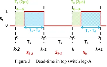
In order to adapt the proposed inductance estimation method to practical converter implementation, the presence of dead-times in the devices switching needs to be taken into account. In fact, as described in section IV, the proposed method considers the switching signals for each leg of the converter and the dc-link voltage. However, switching dead-times (Td region in Figure 3), considered equal to 2µs in this work, results in a voltage drop which affects the estimation method. Therefore, this voltage drop needs to be compensated. A dead-time compensation method has been included in the model predictive control by incorporating an additive term representing the voltage drop due to the dead time Td. The voltage loss in the ‘Td’ region for interval Sk for leg A is expressed as
WX, 13 ∙ W ∙88 ∙ 2YX$ & YZ$ & YW$ & 19
WX, , 13 ∙ W ∙8 88 ∙ 2YX$ YZ$ YW$ 20
Therefore, the total converter voltage applied during the sampling interval Sk is now expressed as
WX[$ WX, ) WX, , 21
[image:4.595.344.512.209.334.2]Similarly, (19)–(21) are applied for the other legs with reference to the direction of the supply currents in the respective legs [23]. The converter voltages are hence transformed to their respective α and β components to be used in the current predictions for (3) and (6) and for the inductance estimation method, (24) and (25).
Figure 3. Dead-time in top switch leg-A
IV. INDUCTANCE ESTIMATION METHOD
[image:4.595.81.262.273.386.2]The estimation method proposed in this paper estimates the total inductance, i.e. supply inductance plus converter inductance, and feeds the estimated value as an update to the model based predictive controller, as shown in Figure 4. Using the total estimated inductance value, we can easily find the variation in supply inductance, LS, and make an estimation of the supply/grid voltage inside the controller.
Figure 4. Block scheme of proposed MPC with online inductance and grid voltage estimation
According to [26], since the voltage harmonic magnitude decreases as the frequency increases, the effect of high frequency harmonics on the grid impedance are often limited in power systems. Moreover, the predictive control does not
seem to be significantly affected by high frequency components of grid impedance, thanks to its inherent robustness. Therefore, it is reasonable to assume a low frequency grid impedance model [26]. Referring to Figure 5, the estimation approach works on the principle of assuming a constant grid voltage magnitude between two consecutive sampling instants. Although there will be a phase shift of ‘ω·ts,’ the magnitude of the grid voltage vector will, however, not vary significantly.
Figure 5. Grid voltage representation in α-β.
In α-β reference frame, the square of the grid voltage magnitude at the instant k is expressed as
U $U: @ A$C:) @ B$C: 22
According to Figure 2 and Figure 5, the grid voltage magnitude at the time instant k can be expressed using the value of vgridk extracted from the system model in α-β:
@ $C: ∙ ) ∙ $) $ : 23
Hence, the square of the grid voltage magnitude at instant
k is expressed as:
U $U: ∙ A) ∙ A$)
A$
:
) \ ∙ B) ∙ B$) B$] :
24
Similarly, the square of the grid voltage at the previous instant, k – 1, is equated as:
U $ &U: ∙ A) ∙ A$ &) A$ &
:
) \ ∙ B) ∙ B$ &) B$ &] :
25
[image:4.595.55.289.487.654.2]dc-link voltage. After discretizing the current derivatives, (24) and (25) are solved for the value of the total inductance
L such that:
U $U: U $ &U: 0 26
This resulted in the quadratic equation of (27), with the terms A, B and C expressed, respectively, by equations (28)-(30) with the single terms defined in (31)- (33).
:∙ ^ ) ∙ _ ) ! 0 27
^ ∆^A& :) @∆^B&C: ∆^A: : @∆^B:C: 28
_ 2 ∙ @∆_A&∙ ∆^A&) ∆_B&∙ ∆^B&
∆_A:∙ ∆^A: ∆_B:∙ ∆^B:C 29
! ∆_A& :) @∆_B&C: ∆_A: : @∆_B:C: 30
∆^A& A
$%&
A$
8a , ∆^B& B $%&
B$
8a ,
∆^A: A $
A$ &
8a , ∆^B: B $
B$ &
8a 31
∆_A& A$) 2A$, ∆_B& B$) 2B$ 32
∆_A: A$ &) 2A$ &, ∆_B: B$ &) 2B$ & 33
After substituting (28)-(30) in (27), the total inductance is evaluated as
= T bMT Lc 12 ∙_^ ∙ d 1 ) P1 4 ∙ ! ∙ ^_: e 34
The estimated value of inductance in (34), once excluded the negative root, is used as an update to the inductance value in the current predictions of (3) and (6).
V. GRID VOLTAGE ESTIMATION
If the voltage at the point of common coupling vpcc presents substantial distortion and it is used in the model, it will in turn induce distortion on the current predictions. We need therefore an estimation of the grid voltage. Once the total inductance has been estimated the supply inductance LS is estimated as:
f[ = T bMT Lc 2 35
[image:5.595.331.517.391.494.2]where, the value of LC is usually known since it is the converter input inductance. Referring to the block diagram in Figure 4, the supply voltage in αβ reference frame used for the predictive controller is corrected using the estimation in (35):
' A,B$ f[∙ A,B $%&
A,B$
8a ) < A,B$ 36
where, -g,h
ijk -g,hi
, is the discretized supply current
derivative and vpccαβk is the actual measurement of the voltage at PCC. Using the ' A,B$and l[ in (3) and (6) for current predictions, it is possible to apply the previously described MP-DPC in a way that the resultant control action takes into account supply impedance variations and the system performance is not affected. In cases when the grid has a low SCR, i.e. very high grid inductance, a phase shift between the supply current and vpcc is present in addition to the distorted vpcc. Moreover, the fundamental component of vpcc does not accurately approximate vgrid because of the variable grid inductance, thus resulting in a phase and magnitude error with respect to vgrid. Therefore, estimating the grid voltage is much more efficient and suitable, particularly in a low SCR scenario.
VI. SIMULATION RESULTS
The proposed MP-DPC is applied to the three-phase two level AFE of Figure 1 with the system parameters reported in table I. Simulation results obtained in Matlab-Simulink environment are shown and discussed in this section.
TABLE I. SIMULATION PARAMETERS
Parameter Symbol Value
PCC voltage vPCC 100Vrms
Sample time Ts 50µs
Converter filter inductance Lc 4.5mH Converter filter resistance r 0.4Ω
Active Power P 2400W
DC-link capacitance C 2200µF Weighting factors S1, S2, S3 1.5, 1, 1 Average switching frequency FSW 9.7 kHz
Although the converter has an average switching frequency, [11], of ~9.7 kHz, the sample time used for the predictive control is fixed at 20 kHz. Figure 6 shows the estimated inductance and its reference value, where the method has been tested in the extreme condition of a frequent variation in LS. The estimation algorithm evaluates the total inductance quite accurately even when the supply inductance LS has been varied in order to reach a value greater than 200% of LC.
Figure 6. Estimated Total Inductance with a variation in LS, LC =4.5mH
0.2 0.4 0.6 0.8 1 1.2 1.4 1.6 1.8 2
5 6 7 8 9 10 11 12 13 14 15 16
Time (s)
In
d
u
c
ta
n
c
e
(
m
H
)
[image:5.595.309.541.601.722.2]In terms of system SCR, results are shown in table II, where the SCR has been defined as [27]:
Y!" Yℎq_Xau ?qtu (Y W Wr sqtu (Y!?)
vw[x)
(37)
The estimation method proposed in this paper works effectively for SCR values larger than 2, at which the system starts showing an unstable behavior.
TABLE II. SCRVALUES FOR DIFFERENT LS VALUES
LS
(mH) LC
(mH)
ZS (Ω) SCP
(kVA) SBASE
(kVA) SCR
1.0 4.5 0.314 95.47 2.4 39.8
2.0 4.5 0.628 47.77 2.4 19.93 4.0 4.5 1.257 23.86 2.4 9.954 6.0 4.5 1.885 15.91 2.4 6.637 8.0 4.5 2.513 11.94 2.4 4.98
10.0 4.5 3.142 9.55 2.4 3.98
12.0 4.5 3.770 7.96 2.4 3.32
[image:6.595.48.286.224.317.2]Figure 7 shows total inductance and grid voltage estimation results for the case when LS is 3.0mH and the converter input filter inductance is 4.5mH. The same value of LS has been used in the experimental results section. The supply voltage used for the predictive controller is corrected by using the estimated value of the supply inductance where the PCC voltage and grid voltage estimation have a THD of ~18% and 1.16% respectively.
Figure 7. Actual vPCC, vgrid-estimation, current, L-est. LS = 3.0mH Figure 8 shows the supply current and estimated grid voltage for a step variation of 3.0mH in LS from 0.5mH to 3.5mH at 0.09s.
Figure 8. vGRID estimation and Current– LS= 0.5mH 3.5mH
When the LS is 0.5mH, the current THD is ~5.48%. Due to the large mismatch between the real and the model value of LS at 0.09s because of the step change, the control and estimator performance gets affected, boosting the THD to 22.35%. However, once the estimator has reached a steady state within a fundamental period, the corrected values of LS and grid voltage largely improve the control performance achieving a current THD of ~3.66%.
Table III shows the THD of the supply current for different variations in LS when the grid voltage has also been estimated. Once the LS is correctly estimated, the increase in the total inductance on the AC side obviously improves the quality of the current waveform, as it can be seen from the reduction of THD values from 5.48% (LS = 0.5mH) to 3.18%
(LS = 5.0mH) in the case of online estimation. Thus,
presenting highly improved performance.
TABLE III. CURRENT THDS :ESTIMATION TO VARIATION OF LS
LS (mH) LC (mH) THD(%)
0.5 4.5 5.48
1.0 4.5 4.93
2.0 4.5 4.29
3.0 4.5 3.76
4.0 4.5 3.39
5.0 4.5 3.18
VII. EXPERIMENTAL RESULTS
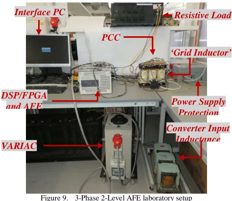
[image:6.595.313.502.284.385.2]Experimental tests have been carried out using the laboratory setup as shown in Figure 9. The experimental implementation uses circuit configuration and data as in simulation.
Figure 9. 3-Phase 2-Level AFE laboratory setup
The control system is composed of a main board featuring a TMS320C6713 digital signal processor (DSP) with 225MHz clock frequency and an auxiliary board equipped with a field programmable gate array (FPGA)
ActelProASIC3A3P400 used for data acquisition and PWM
generation with 50MHz clock frequency. The experimental tests have been carried out using a controlled pure sinusoidal voltage power supply manufactured by Chroma
0.02 0.03 0.04 0.05 0.06 0.07 0.08 0.09 0.1 0.11
-150 -100 -50 0 50 100 150
V
o
lt
a
g
e
(
V
),
C
u
rr
e
n
t*
3
(
A
)
Vpcc V-grid estimation Supply Current
0.025 0.03 0.04 0.05 0.06 0.07 0.08 0.09 0.1 0.11 0.12
6 7 8 9 10
Time (s)
In
d
u
c
ta
n
c
e
(
m
H
) Lreference Lestimation
0.06 0.07 0.08 0.09 0.1 0.11 0.12 0.13 0.14
-150 -100 -50 0 50 100 150
Time (s)
V
o
lt
a
g
e
(
V
),
C
u
rr
e
n
t*
3
(
A
)
Vpcc V-grid estimation Supply Current
THDi = 5.48% THDi = 22.35% THDi = 3.66%
Weak grid Stiff grid
Interface PC
VARIAC
Resistive Load
Power Supply Protection ‘Grid Inductor’ PCC
DSP/FPGA and AFE
[image:6.595.306.543.435.640.2](Programmable AC Source 61511) and also using a VARIAC (Variable Voltage Auto-Transformer CMV20E-3) connected with the mains. In figure 9 the experimental rig is powered through a VARIAC autotransformer, which is connected to a power supply protection circuit in case of over-current or short-circuits in the system. The power supply protection is then connected to a three phase inductor emulating the unknown grid inductance, shown as LS in figure 4, with 3mH per phase. Measurements of supply voltages for data processing are taken at the point of common coupling, PCC, after the grid inductance. A converter inductance of 4.5mH per phase, LC as shown in figure 4, is connected between the PCC and the AFE input and is known to the converter control. The AFE is controlled using the above mentioned DSP/FPGA structure connected to an interface PC, as shown in figure 9. The estimation algorithm is executed in c-code in the DSP and run following the procedure presented in (28)-(33) where, after calculation of each of the terms ∆^A&, ∆^A:, ∆^B&, ∆^B:, ∆_A&, ∆_A:,
∆_B& and ∆_B: in (31)-(33), they are substituted in (28)-(30) for calculation of the terms A, B and C. The terms A, B and
C, are then substituted in (34) to obtain the estimated value
of total inductance. The total computation time required by the algorithm, including control and estimation routines, is ~43µs for an interrupt time of 50µs.
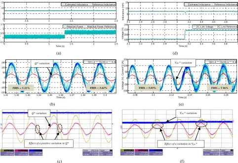
The experiments for the proposed inductance estimation have been carried out both in steady state and transient conditions. That includes a 500VAR variation in reactive power reference, 35V variation in DC-Link voltage reference and also a 67V variation in the supply voltage when the VARIAC is used. The estimation results show a good behavior even in the presence of these variations. Figure 10 shows an experimental test where the Chroma voltage supply was used. In Figure 10 (a), the reactive power was varied from 0VAR to 500VAR and the system is required to estimate a supply inductance of LS=3.0mH for a total line inductance of L=7.5mH. The reactive power follows the requested change and the inductance estimation responds very well to this condition too. However, a very small steady state error of ~50VAR can be seen on the reactive power. This is due to the presence of ripple on the estimated inductance, effect of mutual inductance on the transmission line, other parameter uncertainties and model discretization errors that have not been compensated. The corresponding results in Figure 10(b) show the distorted measured PCC voltage, the estimated grid voltage and the quasi-sinusoidal supply current with a THD value of 5.31%. Figure 10(c) shows the oscilloscope results for the CHROMA supply voltage, supply current and the dc-link voltage when a reactive power variation of 500VAR occurs. Figure 10(d) shows the test results and estimation results in the case of a 35V step in the dc-link voltage reference. The dc-link voltage responds to this reference variation and so does the estimated inductance for the same LS and LC values as for reactive power variation. Since in an active front end the exchange of power is between the AC side and DC side, increasing the dc-link voltage reference essentially means the supply current is increased as well. This is shown in Figure
10(e) where the amplitude of current increases due to an increase in link voltage. Despite this large variation in dc-link voltage reference, the grid voltage shows a good estimation even though the PCC voltage remains distorted. The supply current shows a small variation in THD from 5.03% before the step to 5.96% after the step in dc-link voltage reference. Figure 10(f) shows the oscilloscope results for CHROMA supply voltage, supply current and the dc-link voltage to a variation in dc-link voltage reference. The increase in the supply current amplitude and also the dc-link voltage can be seen in figure 10(f). When figure 10 is compared with the simulation results of figure 7 an increase of ~1.5% in the supply current THD value can be noted. This is caused by parameter uncertainties like, for example, power switching device voltage drop that have not been taken into account in the simulation. The vpcc and vgrid-est have ~17% and ~2.7% THD values, respectively. Figure 11 shows the results for the case when the system is supplied by the mains through a VARIAC. At time 0.55s, a step in input voltage from 33V to 100V was introduced using the VARIAC. This operation changes the VARIAC built-in inductance generating an increase in the total system input inductance from 7.5mH to approximately 8.3mH as estimated by the algorithm and shown in Figure 11.
This means that the mismatch between the supply inductance and the converter input inductance is increased from 66.67% to 85%. Moreover, it has been noted that, considering the small sampling time of the control/estimation algorithm with respect to the dynamics of eventual variations of Ls or supply voltage in a real scenario, imposing constant magnitude of vgrid and considering Ls constant between two sampling intervals, does not cause any uncertainty in the estimation process
.
Due to laboratory safety reasons, the tests were not conducted for higher supply inductance values; however, the simulation and practical results shown support the proposed methodology. The effect of capacitance on the transmission line has not been taken into consideration in the proposed estimation algorithm. Since the effect of capacitance appears at high frequency, its presence will not have a significant effect on the estimation algorithm since the fundamental frequency of the power system is 50Hz.
VIII. CONCLUSION
performance. Estimating the variation in grid inductance allows an estimation of the grid voltage inside the controller so that the vpcc can be updated at each sampling interval for a better quality operation. Though the system in Figure 1 has been tested considering vgrid is from a low voltage substation, the proposed algorithm can be easily adapted and modified to be used for general supply impedance estimation, medium or high voltage applications. The algorithm is also easily
adaptable in the case of any topology of grid connected converters, PV applications, variable load on the distribution network or in the case of a different grid connection like for example the use of LCL filters. The estimation approach has been integrated within the model based predictive control, thus making the estimation and control effective and efficient. Simulation and experimental results support the proposed methodology.
(a) (d)
(b) (e)
(c) (f)
Figure 10. (a) Estimated Total Inductance and reactive power with a variation in Q*, (b) PCC Voltage, Grid Voltage estimation, Supply Current with a variation in Q*. LC = 4.5mH, LS = 3.0mH, (c) Scope result for CHROMA voltage (yellow), supply current (pink) and dc-link voltage (blue) with a variation
in Q*, (d) Estimated Total Inductance and VDC with a variation in VDC*, (e) PCC Voltage, Grid Voltage estimation, Supply Current with a variation in VDC*.
LC = 4.5mH, LS = 3.0mH, (f) Scope result for CHROMA voltage (yellow), supply current (pink) and dc-link voltage (blue) with a variation in VDC*
(a) (b)
Figure 11. (a) Estimated Total Inductance, PCC voltage, grid voltage estimation and supply current with a variation in VARIAC, (b) Zoomed in PCC Voltage, Grid Voltage Estimation, Supply Current
0 0.5 1 1.5 2 2.5
0 5 10 15 In d u c ta n c e ( m H )
Estimated Inductance Reference Inductance
0 0.5 1 1.5 2 2.5
-0.5 0 0.5 1 1.5 Time (s) Q (k V a r)
Reactive Power Reactive Power Reference
2.2 2.4 2.6 2.8 3 3.2 3.4 3.6 3.8 4
0 5 10 15 In d u c ta n c e ( m H )
Estimated Inductance Reference Inductance
2.2 2.4 2.6 2.8 3 3.2 3.4 3.6 3.8 4
180 200 220 240 Time (s) V o lt a g e ( V
) DC-Link Voltage DC-Link Reference
1.31 1.32 1.33 1.34 1.35 1.36 1.37 1.38 1.39 1.4
-150 -100 -50 0 50 100 150 Time (s) V o lt a g e ( V ), C u rr e n t* 3 ( A
) Vpcc-a Vg-est-a is-a
3.08 3.1 3.12 3.14 3.16 3.18
-100 -50 0 50 100 150 Time (s) V o lt a g e ( V ), C u rr e n t* 3 ( A
) Vpcc-a Vg-est-a is-a
0 0.2 0.4 0.6 0.8 1 1.2 1.4 1.6 1.8 2
0 5 10 15 In d u c ta n c e ( m H
) Estimated Inductance
0 0.2 0.4 0.6 0.8 1 1.2 1.4 1.6 1.8 2
-100 -50 0 50 100 Time (s) V o lt a g e ( V ), C u rr e n t* 3 ( A )
Vpcc-a Vg-est-a is-a
A
B
0.29 0.3 0.31 0.32 0.33 0.34
-40 -20 0 20 40 Time (s) V o lt a g e ( V ), C u rr e n t* 3 ( A
) Vpcc-a Vg-est-a is-a
1.17 1.18 1.19 1.2 1.21 1.22
-100 -50 0 50 100 Time (s) V o lt a g e ( V ), C u rr e n t* 3 ( A
) Vpcc-a Vg-est-a is-a
A
B
THDi = 8.3%
THDi = 6.3%
Q* variation VDC* variation
Effect of a variation in VDC*
Effect of a positive variation in Q* variation
THDi = 5.31% THDi = 5.62% THDi = 5.03% THDi = 5.96%
[image:8.595.60.542.198.528.2] [image:8.595.84.517.579.713.2]9 REFERENCES
[1] J. R. Rodriguez, J. W. Dixon, J. R. Espinoza, J. Pontt, P. Lezana. “PWM regenerative rectifiers: state of the art”, IEEE
Trans. Ind. Electr., volume 52, no. 1, pp. 5-22, (Feb. 2005).
[2] J. N. Reddy, M. K. Moorthy, D. V. A. Kumar. “Control of grid connected PV cell distributed generation systems”, IEEE
TENCON 2008 Conference, pp. 1-6, (Nov. 2000).
[3] V. S. Tejwani, P. V. Sandesara, H. B. Kapadiya, A. M. Patel. “Power electronic converter for wind power plant”, ICCEET
2012 Conference, pp. 413-423, (March. 2012).
[4] S. Kwak, H. A. Toliyat. “Design and rating comparisons of PWM voltage source rectifiers and active power filters for AC drives with unity power factor”, IEEE Trans. Power
Electr., volume 20, no. 5, pp. 1133-1142, (Sept. 2005).
[5] P. Zanchetta, P. Cortes, M. Perez, J. Rodriguez, C. Silva. “Finite state model predictive control for shunt active filters”,
IECON 2011- 37th Annual Conference on IEEE Industrial
Electronics Society, pp. 581-586, (Nov. 2011).
[6] K. Ilango, P. V. Manitha, M. G. Nair. “An enhanced controller for shunt active filter interfacing renewable energy source and grid”, IEEE Third Intl. Conf. on ICSET, pp. 305-310, (Sept. 2012).
[7] M. P. Kazmeirkowski, F. Blaabjerg, R. Krishnan. “Control in power electronics, selected problems”, Elsevier science, pp. 444, ISBN : 0-12-402772-5. USA 2002.
[8] M. Malinowski, M. P. Kazmeirkowski, A. M. Trzynadlowski. “A comparative study of control techniques for PWM rectifiers in AC adjustable speed drives”, IEEE
Trans. Power Elect., volume 20, no. 5, pp. 1133-1142, Sept.
2005.
[9] S. Vazques, J. I. Leon, L. G. Franquelo, J. Rodriguez, H. A. Young, A. Marquez, P. Zanchetta, “Model Predictive Control: A review of Its Applications in Power Eectronics”,
IEEE Magazine, vol. 8, no. 1, pp. 16-31, March 2014
[10] P. Zanchetta, J. Rodriguez, M. P. Kazmeirkowski, J. R. Espinoza, H. A. Abu-Rub, H. A. Young, C. A. Rojas. “State of the art of finite control set model predictive control in power electronics”, IEEE Trans. Informatics, volume 9, no.2, pp. 1003-1016, May. 2013.
[11] J. Rodriguez, P. Cortes. “Predictive control of power converters and electrical drives”, John Wiley & Sons, Ltd, ISBN : 978-1-119-96398-1, 2012.
[12] J. Rodriguez, J. Pontt, C. A. Silva, P. Correa, P. Lezana, P. Cortes, U. Amman. “Predictive current control of a voltage source inverter”, IEEE Trans. Elect., volume 54, no.1, pp. 495-503, Feb. 2007.
[13] P. Correa, J. Rodriguez, I. Lizama, D. Andler. “A predictive control scheme for current-source rectifiers”, IEEE Trans.
Elect., volume 56, no.5, pp. 1813-1815, 2009.
[14] M. P. Kazmeirkowski, L. Malesani. “Current control techniques for three-phase voltage-source pwm converters: A survey”, IEEE Trans. Elect., volume 45, no.5, pp. 691-703,Oct. 1998.
[15] D. E. Quevedo, R. P. Aguilera, M. A. Perez, P. Cortes. “Finite control set MPC of an AFE rectifier with dynamic references”, IEEE Technology, pp. 1265-1270, March. 2010. [16] P. Cortes, J. Rodriguez, P. Antoniewicz, M. P.
Kazmeirkowski. “Direct power control of an afe using predictive control”, IEEE Trans. Elect., volume 23, no.5, pp. 2516-2523, Sept. 2008.
[17] M. Sumner, B. Palethorpe, D. W. P. Thomas, P. Zanchetta, M. C. Piazza. “A technique for power supply harmonic impedance estimation using a controlled voltage disturbance”, IEEE Trans. Electron. volume 17, no. 2, pp. 207-215, March 2002.
[18] A. V. Timbus, P. Rodriguez, R. Teodorescu, M. Ciobotaru. “Line impedance estimation using active and reactive power variations”, IEEE Power Electron., pp. 1273-1279, June 2007.
[19] P. Antoniewicz, M. P. Kazmeirkowski. “Virtual-flux-based predictive direct power control of ac/dc converters with online inductance estimation”, IEEE Trans. Electron., volume 55, no. 12, pp. 4381-4390, Dec. 2008.
[20] J. G. Norniella, J. M. Cano, G. A. Orcajo, C. Garcia, J. F. Pedrayes, M. F. Cabanas, M. G. Melero. “Analytic and iterative algorithms for online estimation of coupling inductance in direct power control three-phase active rectifiers”, IEEE Trans. Electron., volume 26, no. 11, pp. 3298-3307, Nov. 2011.
[21] J. G. Norniella, J. M. Cano, G. A. Orcajo, J. F. Pedrayes, M. F. Cabanas, M. G. Melero. “New strategies for estimating the coupling inductance in grid-connected direct power control-based three-phase active rectifiers”, IEEE PES., pp. 1-5, July. 2013.
[22] M. Ciobotaru, R. Teodorescu, F. Blaabjerg. “A New Single-Phase PLL Structure Based on Second Order Generalized Integrator”, PESC ’06, pp. 1-6, June. 2006.
[23] Seon-Hwan Hwang, Jang-Mok Kim. “Dead-time Compensation method for Voltage-Fed PWM inverter”,
Energy Converter, IEEE Trans., volume 25, no.1, pp. 1-10,
March. 2010.
[24] B. Arif, L. Tarisciotti, P. Zanchetta, J. Clare, M. Degano, “Integrated grid inductance estimation technique for Finite Set Model Predictive Control in grid-connected converters”,
ECCE 2014, IEEE, pp. 5797-5804, Sept. 2014.
[25] M. M. Canteli, A. O. Fernandez, L. I. Enguiluz, C. R. Estebanez, “Three-phase adaptive frequency measurement based on Clarke’s transformation”, Power Delivery, IEEE
Trans., volume 21, no. 3, pp. 1101-1105, July 2006
[26] Gu Herong, Guo Xiaoqiang, Wang Deyu, Wu Weiyang, “Real-time grid impedance technique for grid-connected power converters”, Ind.Electr., ISIE 2012, pp 1621-1626, May 2012
10
Bilal Arif completed his undergradute degree (BEng (hons.)) from the University of Nottingham in the field of Electrical and Electronics engineering in July of 2011. In September 2011, Bilal started his Ph.D. study with the Power Electronics Machines and Controls (PEMC) group at the University of Nottingham, UK. Currently he is in the final stages of his Ph.D. and his research interests include control strategies for grid connected converters with special emphasis on grid impedance estimation techniques for cases when power converters are connected to weak grids that have low short circuit ratio values.
Luca Tarisciotti received the Master’s degree in electronic engineering from The University of Rome "Tor Vergata" in 2009 and his Ph.D. degree in electrical and electronic engineering in the PEMC group, University of Nottingham in 2015. He is currently working as Research Fellow at the University of Nottingham, UK. His research interests include multilevel converters, advanced modulation schemes, and advanced power converter control.
Professor Pericle Zanchetta received his degree in Electronic Engineering and his Ph.D. in Electrical Engineering from the Technical University of Bari (Italy) in 1993 and 1997 respectively. In 1998 he became Assistant Professor of Power Electronics at the same University and in 2001 he joined the PEMC research group at the University of Nottingham – UK, where he is now Professor in Control of Power Electronics systems. He is Vice-chair of the IAS Industrial Power Converters Committee (IPCC) and Associate Editor of the IEEE Transactions on Industry Applications and IEEE Transactions on Industrial Informatics.
Jon C. Clare (M’90–SM’04) was born in Bristol, U.K. He received the B.Sc. and Ph.D. degrees in electrical engineering from the University of Bristol, U.K. From 1984 to 1990, he was a Research Assistant and Lecturer at the University of Bristol involved in teaching and research in power electronic systems. Since 1990 he has been with the Power Electronics, Machines and Control Group at the University of Nottingham, U.K., and is currently Professor in Power Electronics and Head of Research Group. His research interests are power electronic converters and modulation strategies, variable speed drive systems, and electromagnetic compatibility.