Development of a Tool Cost Optimization Model for Stochastic Demand of Machined Products

(1)

ISSN Online: 2152-7393 ISSN Print: 2152-7385

DOI: 10.4236/am.2018.912091 Dec. 28, 2018 1395 Applied Mathematics

Development of a Tool Cost Optimization

Model for Stochastic Demand of

Machined Products

Francisco G. Pantoja

1

, Victor Songmene

1

, Jean-Pierre Kenné

1

, Oluwole A. Olufayo

1

,

Michael Ayomoh

2

1_{Mechanical Engineering Department, École de Technologie Supérieure (ÉTS), Montreal, Canada} 2_{Industrial and Systems Engineering Department, University of Pretoria, Pretoria, South Africa}

Abstract

Cutting tool management in manufacturing firms constitutes an essential element in production cost optimization. In order to optimize the cutting tool stock level while concurrently minimizing production costs, a cost optimiza-tion model which considers machining parameters is required. This inclusive modeling consideration is a major step towards achieving effectiveness of cutting tool management policy in manufacturing systems with stochastic driven policies for tool demand. This paper presents a cost optimization model for cutting tools whose utilization level is assumed to be optimized in respect of the machining parameters. The proposed cost model in this re-search incorporated the effects of diversified machining costs ranging from operational through machining, shortage, holding, material and ordering costs. The machining of parts was assumed to be a single cutting operation. Holt-Winters forecasting technique was used to create a stochastic demand dataset for a test scenario in the production of a high-end automotive part. Some numerical examples used to validate the developed model were imple-mented to illustrate the optimal machining and tool inventory conditions. Furthermore, a sensitivity analysis was carried out to study the influence of varying production parameters such as: machine uptime, demand and cutting parameters on the overall production cost. The results showed that a desired low level of tool storage and holding costs were obtained at the optimal stock levels. The machining uptime had a significant influence on the total cost while tool life and cutting feed rate were both identified as the most influenti-al cutting variables on the totinfluenti-al cost. Furthermore, the cutting speed rate had a marginal effect on both costs and tool life. Other cost variables such as shortage and tool costs had significantly low effect on the overall cost. The

How to cite this paper: Pantoja, F.G., Songmene, V., Kenné, J.-P., Olufayo, O.A. and Ayomoh, M. (2018) Development of a Tool Cost Optimization Model for Stochas-tic Demand of Machined Products. Applied Mathematics, 9, 1395-1423.

https://doi.org/10.4236/am.2018.912091

Received: November 12, 2018 Accepted: December 25, 2018 Published: December 28, 2018

(2)

DOI: 10.4236/am.2018.912091 1396 Applied Mathematics

output trend showed that the feed rate is the most significant cutting para-meter in the machining operation, hence influencing the cost the most. Also, machine uptime and demand significantly influenced the total production cost.

Keywords

Inventory, Tool Cost Optimization, High Value Product, Stochastic Demand, Machining Parameters

1. Introduction

Research in the field of cost optimization modelling for stochastic inventory management and control has significantly intensified over the past few decades

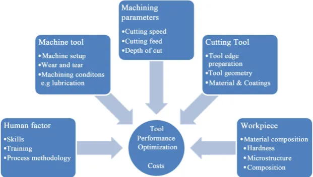
[image:2.595.218.529.528.704.2]

[1]. The ability to minimize the overall production cost of a machining process while adapting to the ever growing levels of stochasticity in the open market can be considered a major step towards its competitiveness. This capability must, however occur without adversely affecting throughput and production quality amidst multiplicity of inherent market conditions. Machining operations gener-ally constitute a large segment in the manufacturing sector with costing effec-tiveness serving as a critical success factor. In a machining process, the cutting tool represents an essential element to the entire machining system. This is so because its effect is directly linked to a multiplicity of factors such as: the quality of finished product, cycle time of operation and ultimately the cost of machining amongst others. The significance of the influence of machining parameters on the cutting tool, workpiece and other machining components during an opera-tion is quite crucial to deciding the overall producopera-tion cost. Some notable com-ponents that make up an ideal machining operation are as presented in Figure 1. The optimum behavior of a machining operation can be influenced by any one of these member elements.

(3)

1.1. Predictive Challenges to Manufacturing

Companies that focus on industrial metal works are often faced with predictive challenges even though there are several quantitative techniques that can be used to improve production processes such as forecasting, probability distributions and optimization related methods amongst others [2]. Very often, applicability within this research space can be limited hence, resulting in a significant pro-duction planning problem. Some of these problems are traceable to inefficiencies in the administrative and production processes derived from a poor strategic planning.

In most companies, the behavior of product sales is random, since it is diffi-cult to absolutely predict demand to determine sales. Due to this challenge, the focus is often placed on alternate areas where the lack of a sound process design can be mitigated and controlled. Some of these areas include:

 Production: The lack of a future programming and being left with the expec-tation of the needs of the clients, manufacturing companies are forced to ful-fill the demand of their clients by incurring additional time in the productive processes.

 Inventories. To the poor management of inventory levels, such as the case of high inventory level, this causes high costs and prevents the expansion of the business.

 Finances: Given the high costs of inventories, companies limit their growth in the purchase of new equipment to make production processes more effi-cient.

To mitigate these and other problems caused by poor planning of the produc-tion, it is necessary to design a methodology that provides accurate predictions of the sales of industrial metal mechanical products or mitigate alternate costs generated elsewhere in production [3]. Actual modeling of industrial systems is complicated because of the variability of factors, in many cases it is necessary to make complex combinations of several distribution functions to resolve such problems.

1.2. Optimization Modelling in Manufacturing

Existing machining models more often than not, are seen to be analyzing the combination of different cutting materials by focusing on their conditions while conducting analytical, numerical, empirical and artificial intelligence based ob-servations. Robust predictive models are often required to accommodate the complex interaction that exists amongst the trio of a workpiece, the cutting tool and the machine tool [4] [5] [6] [7].

(4)

stress, strain rate and temperature amongst others. From the point of view of demand, when a product with intricate properties such as high strength (e.g. aerospace superalloys) is seasonally or randomly produced, it often becomes dif-ficult for industries machining these materials to adequately estimate the quan-tity of cutting tools needed to meet the demand. On the other hand, working with high strength materials increases the tendency of tool penalty cost due to short tool life. These effects are central to the increase in the cost of products and a reduction in the overall profit margin. These costs could be associated with storage costs, ordering costs, stock-out or shortage costs.

1.3. Recent Studies on Cost Optimization in Machining

Traditional procurement policies are subjective and often premised on periodic supply decisions. These policies are usually based on simplified and idealistic assumptions, as well as on the expected cost criterion, without considering ma-chining factors as well as the finished goods throughput. Some research works

[8] [9] [10] [11] [12] have considered more inclusive views into production cost in manufacturing by considering machining conditions. However, the need for a more generalized and adaptable model based on a stochastic demand is needed to optimize production cost in the manufacturing sector.

The rate of tool depletion was found to be a function of tool life and machin-ing conditions. Findmachin-ing the optimal machinmachin-ing conditions related to tool life and obtaining the optimal order quantity could stabilize cycle length and ordering cycle. A study into production cost in the milling of titanium alloys by consi-dering machining conditions, was conducted by Conradie, Dimitrov and Oos-thuizen [12]. In their paper, they designed a cost model which considered pre-cost of manufacturing and auxiliarycost incurred based on machining pa-rameters. Their approach generated means to estimate the cost of titanium mil-ling based on actual machining and pre-manufacturing conditions. Further-more, due to tools supply unpredictability and market demand variability, nu-merous researchers have sought to design models which would be used to max-imize the efficiency in tool management to mitigate the adverse costs incurred in shortage conditions [9] [10] [11].

(5)

In their research work on cost modelling in milling operations, Parent, Song-mene and Kenné [11] used an optimization technique premised on operations research to minimize machining time and evaluate the cost of milling operation hence, demonstrating the practicality of the algorithm in solving cost related problems and as a decision-making aid for a central controller flexible manu-facturing cell. Their approach yet only considers an optimization of the ma-chining cost in the overall production cost and ignores the inventory manage-ment. This approach can be deployed for analysis of the impact of setup time while computing for the capacity of a system emanating from a new design and in determining the manufacturing price of parts.

The above mentioned works, as most resources from the literature, do not consider the attributes that influences the productive length of a tool-life while solving the general optimization problem. It is however important to recognize that the tool-life productive length has a great impact on tool procurement and management of its inventory systems as well as indirectly influence total operat-ing cost.

1.4. Problem Statement

Based on the reality of market variability, which has got so much impact on production processes, modern day manufacturing firms are faced with a rising level of supply uncertainty and demand variability. These fluctuations are char-acterized with challenges capable of impacting negatively on the optimum per-formance level and general sustainability of the manufacturing sector. Industrial firms involved in the production of high-valued parts such as the automotive or aerospace industry amongst others are often posed with these challenges [13]. These firms often seek to identify optimum machining parameters to increase tool life while maintaining a high quality production level. Optimization of ma-chining time as well as tool inventory cost management are key factors for at-taining high production efficiency for these high-value parts. A functional tool optimization policy capable of reducing costs and sustaining the overall tool op-timum conditions has become a major priority in production systems function-ality.

Other factors of significant importance in manufacturing processes include machine unit costs, machine uptime costs, ordering costs and lead-time due to their impact on procurement, tool inventory policy and influences on tool life-span. These considerations if well managed, can reduce the costs associated with production activities, decrease the levels of inventory of tools with low demand and increase the level of service for products considering their seasonality and cyclicality.

(6)

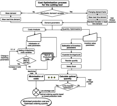
[image:6.595.60.541.265.699.2]

This paper develops a nonlinear cost optimization model based on an inventory policy for cutting tools at optimum machining parameters for the production of high-value mechanical parts. Finally, the study inclusively offers information to a production manager regarding the life of his cutting tools in a production process and permits the flexibility to adapt a production process to suit demands consumer requirements.

Figure 2 shows a flowchart that depicts the overall production cost optimiza-tion process developed in this study. The optimizaoptimiza-tion process carried out using LINGO software utilized a combined modelling effect of cost minimization and optimum quantity computation as presented in Figure 2. This results in a minimized production cost and optimized ordering quantity. However, these are achievable only when the ordering quantity is optimized.

(7)

2. Model Formulation

In this section, the model development is introduced with the mathematical formulations, assumptions and constraints. Prior to the model formulation, an illustration of the interaction between main cost components and effect of cost modelling is presented as seen in Figure 3. Herein, the dynamical relationship amongst cost, productivity and basic machining parameters are presented. The optimization process of the model in this research seeks to find the lowest point on the total cost curve amidst diverse production costs. This point marks the be-ginning of the high efficiency zone in choice of machining parameters where ef-ficient machine and tool life utilization is achieved.

From Figure 3, it could also be seen that the drop in total cost crosses the ris-ing productivity of operations hence, creatris-ing an efficient range in production. A subset of this range was found between the lowest cost and highest productivity for the highest machining efficiency. This range is based on a set of machining parameters which indicates the most favorable machining conditions. Beyond the efficient performance zone, the occurrence of severe tool damage creates a proportionate rise in production costs and drop in productivity. On the other hand, below the optimal machine utilization point, the tool utilization is not maximized hence leading to a reduction in tool costs yet resulting in a relatively high machining costs due to poor efficiency.

2.1. Hypothesis

This sub-section presents the assumptions considered in the model development process:

[image:7.595.210.537.466.693.2]

1) Tool orders are made on request and not in predefined cyclic batches.

(8)

2) The cutting operations tools are mainly divided into two groups, namely: tools for roughing and finishing operations. However, this research will focus on the use a single cutting operation.

3) Once a cutting tool has reached its life span, it is no longer used to avoid tool breakage and the occurrence of a defective process. This also eliminates the penalty cost for tool break.

4) The life span of a tool is considered based on empirical models with the experimentation of similar conditions.

5) Tool vendors are located nearby resulting in a fixed lead time. Hence, all tool demands are satisfied in real-time without any need for back orders.

6) Labor cost is included within machine usage cost and considered to be a constant.

7) Inventory is considered as the average between the initial and final inven-tory.

8) The demand of part product is random, however, it presents patterns of seasonality, cyclic tendencies that can be followed through forecasting methods such as triple exponential smoothening as premised in (Holt-Winter’s Method). Some examples of these patterns are festive yearly seasons, economicfactors, re-cession and inflation.

9) Machine time used is inclusive of both operational, setup and installation time.

10) Price per unit product is constant 11) Ordering costs are constant

12) The holding cost is a constant and includes both the warehouse and pres-ervation costs.

13) Initial purchases are below demand quantity.

Objective Function

The focus of this research is to optimize production by obtaining the minimum total cost of operations supported by the inventory system as a complete manu-facturing process. This can be represented by an objective function which con-sists of the cost optimizations elements, these are; the cost of operations, cost of holding, cost of shortage, annual ordering and raw material costs.

Total cost operational cost shortage cost holding cost raw material ordering cost

= + +

+ +

( )

TC $ =Cop $ +Csh $ +Ch $ +CB $ +Co $

*TC = total cost of production in over a production time period i.

The next sub-sections present the details of the elements of the objective func-tion:

2.2. Cost Optimization Elements

2.2.1. Operational Cost

(9)

during production is defined by the material volume to be cut (Length × Width × Height) and the depths of cut (radial and axial) as presented in Figure 4. A representation of Taylor’s extended tool life model was applied in this research. The machining workpiece in this research is a rectangular prism which requires different operational schedules ranging from rough cuts through smoothened finish cuts. This research would however focus on the rough cut hence a single cutting operation. The decision variables associated with the material removal process include: width of cut (wr and wf), depth of cut (dr and df) and

feeds (vfr and vff).

To estimate the life span of a tool using Taylor’s empirical model as presented in Equation (2), it is necessary to determine the tool cost. The following equa-tions are a derivation of the original Taylor’s model:

0 r

k t

v f d wα β ε =

In application for milling operations, the tool life expression (t0) was

ex-tended by adding the radial width of cut with α, β and ε serving as parametric constants. Equations based on this type of operation could be devised for either roughing or finishing operations i.e. t0r or t0f. However, this research is

fo-cused on the roughing operation as presented in Equation (3) below:

0r

r r r r

k t

v f d wα β γ λ =

The parametric constants defined in this model need to be obtained through experimentation due to the fact that the machining conditions such as the tool material-make, workpiece, cutting fluid, rigidity of the assembly and the system vibration amongst other factors, vary significantly from one machine to the other. These can be determined using a statistical design of experiment (DOE)

[11].

The cost of tools utilization per hour is defined here as the ratio of the current market price to the tool life as presented in Equation (5). The tool life is usually expressed in terms of the operations the tool is subjected to over time:

[image:9.595.298.450.550.694.2]

(10)

DOI: 10.4236/am.2018.912091 1404 Applied Mathematics 0 pr hr r c c t =

In this research, the primary focus is the cutting operation. Apart from iden-tifying and analyzing the cutting operations, a special consideration is also given to the respective quantities of cutting tools (Qp) deployed during the overall

production task. A combination of all these results in the models below: ( ),

operational cost=Cop =cr f ⋅Qp

where,

(

0

)

r opr hr opr

c = k t⋅ +c t⋅

(

0

)

f opf hf opf

c = k t⋅ +c t⋅

(

roughing

)

(

finishing

)

p r f

Q =Q +Q

where Qf =0 in roughing only operations.

Thus:

( )

$

(

0

)

op op hr op p

C = k t⋅ +c t⋅ ⋅Q

2.2.2. Holding Cost

The holding cost represents all the costs associated with the storage of the ventory until its depletion. These costs usually include tied-up capital, space, in-surance, protection, taxes attributed to storage amongst others. The holding cost can be assessed either continuously or on a period-by-period basis. A common consideration for the holding cost is that an initial inventory level exists at the beginning of every period. Based on this, the inventory cost at the beginning of a period I can be obtained from:

( )

$

{

}

h h i s

C

=

c I Q

+

where Ii is considered as the average inventory level required to avoid short-age of cutting tools. This is computed based on the summation of the initial and final inventory levels divided by two.

(

initial final

)

2

i

I I

I = +

Furthermore,

I

i as presented below, represents the total amount of tools required to meet the demand for a given product.

i s i

I Q I

=

+

In addition, considering the likely physical limitations of a warehouse in terms of its holding capacity, the capacity of storage can be represented as:

i i

I

≤

A

Considering that the average inventory, we can add it directly to the objective function as follows:

( )

$

h h i

(11)

DOI: 10.4236/am.2018.912091 1405 Applied Mathematics 2.2.3. Shortage Cost

The shortage cost (Csh) represents the costs incurred during the time produc-tion has a depleted inventory. This is the cost incurred between this time and the period of a re-order. It includes costs of not using the machine and equipment involved in production.

sh sh t

C =c F⋅ ₍₇₎

i t s y F D Q =

where yi service as an indicator for when shortage is present in the equation. It can be activated or switched off during computation and holds two statuses which are 0 or 1. Whereas Ft stands for the amount of missing tools in system.

2.2.4. Material Cost

The material cost of purchasing the workpiece used in production is included for a more inclusive and comprehensive review of the total costs involved in pro-duction. It is a factor of the quantity of material and the cost per unit material purchase.

( )

$

B B B

C

=

Q c

⋅

2.2.5. Ordering Cost

The ordering cost is described as a function of the unit cost of ordering tools, cy-cle time between orders and a variableterm. The variable term zi is used to consider the alternate conditions which are assumed constant in this present model. Such conditions for variability in unit ordering, shipping, delays and al-ternate reasons which could influence this cost could be expanded through this variable in future research modifications of this model. However, in this re-search work, the ordering cost is considered as constant of value 1.

( )

$

O f D i

C C z

Q

=

2.3. Basic Objective Function for Single Operations

The objective function formed to minimize the production cost that involves the operation cost, shortage cost, holding cost, material cost and ordering cost is shown in the Equation (11). The cost of labor is not included in this function. The focal point of this function lies in the operational costs which is derived from the machining parameters and tool conditions.

(

)

MinTC Q T i C_{p c} = _op+C_sh+C C_h+ _B+C_O

(

)

(

0

)

0 0

Minimised Total Cost p, c

i

op hr op p sh i i hi i B B f i s

n

o n

Q T i

y D

k t c t Q c D c I Q c C z

Q Q

= =

= + +

∑

+

∑

+ ⋅ +

2.4. Constraints

(12)

Some decision variables found in the model are the radial width of cut for the roughing operation (wr) and the axial depth of cut (dr). This radial width (wr) is connected to the number of passes and the width of the volume to machine (W):

r w

w N⋅ =W

Also, the axial depth of cut (dr) which is connected to the number of axial passes (Np) and the height (H) of the volume to machine is a decision variable:

r p

d N⋅ =H

Limits are given to the width of radial cuts (wr) by the diameter of the tool (Dt):

r t

w ≤D

The depths of axial cuts (dr) are also limited by the length of the tool flutes (hfmax):

max

r f

d ≤h

Machine-tool constraints

The power needed for the operation relies on the material removal rate (MRR) and the specific power rating of the workpiece material as seen in Equation (12). It can thus be inferred that at maximum machine power, the maximum metal removal rate (MRR) can be determined. This rate depends on the width of cut (wr), the feed ( fr) to the depth (dr), as shown in the equation below:

r r r RR

w f d∗ ∗ ≤M

The material removal rate (MRR) can be denoted as:

( )

maximum machine cutting power

energy coefficent

Unit power for the workpiece material

RR

M ≤ η ⋅ ₍₁₂₎

In this case,

 The cutting speed rate is constrained by the machine’s maximum spindle speed.

max

1000 _;

π tr

v _N

D

⋅ ≤ ⋅

 _{The achievable power is constrained by the maximum safe operational force.}

max

60 r _;

r

HP _F

v

⋅ ≤

 The cutting feed rate is constrained by the machine’s maximum feed rate.

max

r m

f ≤ f

where fmmax is the maximum feed of the machine, Fmax are the maximum

forces obtained from the machine and Nmax is the maximum spindle speed of

the machine.

Inventory and shortage restrictions With restrictions of inventory as follows:

(

Ii−1+Qp

)

− =Ii Q it

i i

(13)

Restrictions of shortage:

t p t

Q Q− =F

( )

0

p i i

Q −I y ≤

Finally, non-negativity is assumed for all the decision variables and binary variables:

, ,

0

t i i

F I A

≥

_and yi =0,1

This project focuses on optimizing the process thought for quantity of tool in an inventory. Therefore the study remains within basic machine limitations or overlooks tool immersion and surface finish as constraints.

3. Solution Methodology and Illustrative Example

The model was implemented in “LINGO” by LINDO® systems. “LINGO” is a commercially available optimization modelling software used for building and solving mathematical optimization models. Its package build-up provides a lan-guage tool needed to build and design models as well as include needed solving tools within a compact integrated environment. It could be applied to linear, nonlinear, quadratic, integer and stochastic optimization problems. A seven core computer with 8 gigabytes of memory was used for the LINDO analysis to minimize processing time. Note that for each result the LINGO solver provided, it declared the solution as being only a local optimum, i.e. it could not fully guarantee a global optimum.

3.1. Graphical Illustration

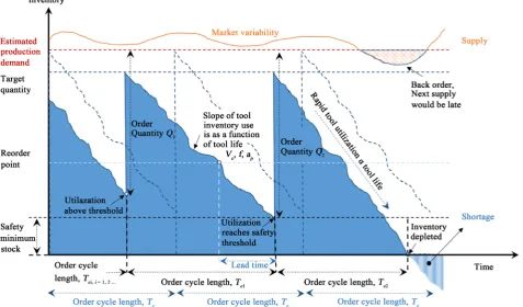
The illustration in below depicts the policy of the model for the annual optimi-zation of production in a manufacturing company whose primary task and op-erations is focused at metal works. This new tool policy includes the forecast of sales and the annual tool planning for production. The main objectives of this illustration is to show how the model can meet a high level of service in sales and a low inventory level of production. As the proposed model is founded on the principle of the Economic order quantity model (EOQ) [15], a generic inventory system adapted to include the influence of machining parameters is produced (Figure 5).

(14)

[image:14.595.61.539.75.355.2]

Figure 5. A generic review inventory system (adapted from Li and Cheng [10], Shang, Tadikamalla, J. Kirsch and Brown [17]) To the other sections. It is a result with more explanantion.

to react to depleting stock. Beyond this threshold the risks of reaching shortage is high.

It is worth noting that a machining tool has an expected productive life around its mean value; therefore, there exists more risk of failure cost for pro-longed use of machining tool over this value. However, a reduction in running time of these tools will potentially increase the replacement quantity and thus re-ordering cost. Therefore, production inventory estimation is contingent on requirement needs based on trends and controlling the utilization time for the tools could be used to regulate the inventory system without influencing the in-tegrity and quality of the product.

3.2. Numerical Sample Case 1

(15)

[image:15.595.208.540.90.173.2]

Table 1. Sample data utilized in numerical example 1; machine constants.

Machine data

Nmax (rpm) 1200 max feed speed 8000

HPs(w/mm3_/min) _59.2 _{max cutting forces (kN)} ₂₀₀₀

Hpmax (kw) 22,000 max spindle speed (rpm) 12,000

Energy efficiency η (%) 0.85

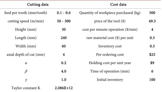
Table 2. Sample data utilized in numerical example 1; cutting parameters, workpiece dimension and cost values.

Cutting data Cost data

feed per tooth (mm/tooth) 0.1 - 0.6 Quantity of workpiece purchased (kg) 500

cutting speed (m/min) 50 - 300 price of the tool ($) 49.5

Height (mm) 30 cost per minute operation ($/min) 4

Length (mm) 240 raw material cost ($) per unit 0.5

Width (mm) 60 Inventory cost 0.5

axial depth of cut (mm) 4 Per ordering cost $25

α 0.2 Holding cost per unit year $9

β 4.0 Time of operation (min) 6

γ 1.0 Initial inventory 100

Taylor constant K 2.086E+12

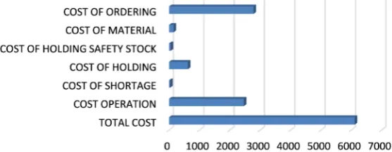
Results and Discussion

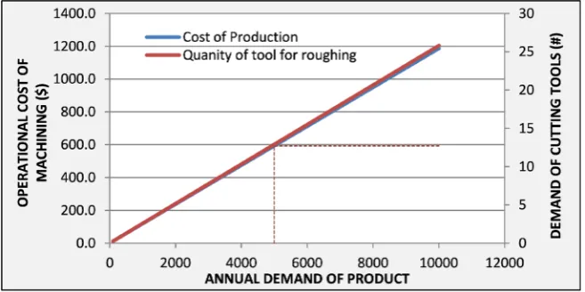
Solving the developed model using the LINGO® solver in Equation (11) gave the following cost breakdown as presented in Figure 6. From the figure, the main contributors to the total production costs were identified as the ordering costs, machine operations costs and holding costs. Ordering costs are known to vary based on the lead-time and unit cost of ordering a tool. As the lead-time to deli-very increased, the ordering costs simultaneously increased. The operational cost on the other hand, is greatly susceptible to changes in tool life. An increment in the amount of tools following a poor performing tool life, was seen to signifi-cantly increase the incurred costs. The model also indicates the significant cost incurred from inventory of tools. Tool quantity stored during the production of the product bares an influence on its selling price. However, due to the success-ful minimization of the model, the separate cost of holding the safety stock as well as the shortage costs has become insignificant in the summation.

This elevated holding cost is due to the short cycle period of 5.5 days for reor-dering. A set of approximately 65 orders per year was obtained. The average forecast quantity of 7 units per order cycle was obtained from Equation (5). This resulted in an optimal order quantity Q0 of about 38 units to minimize total

[image:15.595.210.541.219.406.2]

(16)

[image:16.595.250.511.76.168.2]

[image:16.595.208.538.199.382.2]

Figure 6. Bar chart result of the influence of various costs on total operating cost.

Figure 7. Schematic representation of the order optimization model with added machin-ing op-erational cost.

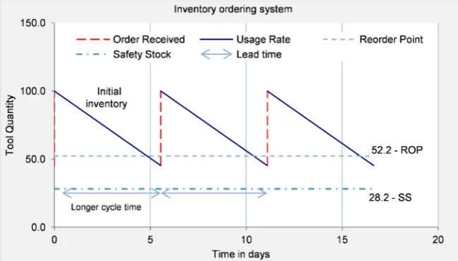
Figure 8. Schematic of inventory control system with a fixed demand.

[image:16.595.210.535.428.613.2]

(17)

3.3. Numerical Sample Case 2

Table 3 summarizes the data used in this numerical sample case 2. This example was adapted from the work of Parent, Songmene and Kenné [11] and modified to suit machining setup proposed in this study. A typical end milling operation of an alloyed steel part (4140, 4340), with a four-flute uncoated high speed steel (HSS) end mill is proposed for evaluation. The diameter of the tool is 19.05 mm (0.375”). The chip load per tooth is estimated to be 0.05 mm/tooth and the speed between 30 - 45 m/min with a hardness between 30 - 38 HRC. The milling ma-chine setup and initialization values, cost parameters as well as parameters for production are listed in the Table 1 & Table 3. The solution represented in this initial part, considers only a fixed demand of 5000 produced parts and deter-mines ideal parameters needed to optimize inventory use and reduce cost. All constraints are established on realistic machine parameters.

[image:17.595.235.514.346.454.2]

Results and Discussion

Figure 9 presents results acquired using the LINGO® solver. The following cost breakdown presented in the Figure 10 was obtained solving the developed model

Figure 9. Bar chart result of the influence of various costs on total operating cost.

Table 3. Sample data utilized in numerical example 2; cutting parameters, workpiece dimension and cost values.

Cutting data Cost data

Cutting feed rate (mm/min) 4.01 Mean Demand/year 5000

feed per tooth (mm/tooth) 0.05 Quantity of workpiece purchased (kg) 200

cutting speed (m/min) 41 price of the tool ($) 90

Height (mm) 25 cost per minute operation ($/min) 4

Length (mm) 100 raw material cost ($) per unit 0.75

Width (mm) 60 Inventory cost 0.5

axial depth of cut (mm) 0.063 Per ordering cost $30

α 5 Holding cost per unit year $6

β 1.75 Time of operation (min) 6

γ 3.5

λ 0

[image:17.595.207.539.518.741.2]

(18)

[image:18.595.209.538.71.235.2]

Figure 10. Schematic representation of tool quantity per order cycle needed at minimum total cost.

in Equation (11). From the figure, the main contributors to the total production costs were identified as the ordering and machine operations cost. However, this example presents a lower inventory holding costs. This is due to the lower cost of purchasing HSS tools and its influence in the combined optimization func-tion. Due to the successful minimization of the model, the holding costs in-curred for safety stock as well as the shortage costs remain insignificant in the overall summation.

For the numerical example, a set of 22 orders per year over an approximate 16 days cycle was obtained. The average forecast quantity of 13 units per order cycle was obtained from Equation (5). This resulted in an optimal order quantity 𝑄𝑄0

of about 54 units to minimize total costs of production. This can also be seen from Figure 11 and Figure 12. The value obtained in contrary to an ideal EOQ model contains the inclusions of the sum of operational, shortage, holding, and material costs. An optimal ordering quantity was obtained at the intersection of the ordering, sum of operations and safety holding costs. The results also indi-cated that a safety stock level of 57 units indicating the least amount in the in-ventory is needed to prevent a shortage situation. Furthermore, a value for re-ordering of stock to match lead time was deduced to be 105 units. An analysis of a controlled inventory system for the numerical example is illustrated in Fig-ure 12.

3.4. Sensitivity Analysis

An in-depth sensitivity analysis of numerical sample case 2 is performed to es-tablish influencing factors relevant to changes in operational costs, determine the influence of demand on inventory optimization and ascertain the key cost drivers of the model using actual industrial stochastic demand data.

3.4.1. Cutting Parameters

(19)

[image:19.595.209.539.74.252.2]

Figure 11. Schematic representation of the order optimization model with added ma-chining op-erational cost.

Figure 12. Schematic of inventory control system with a fixed demand.

most important variables for minimizing this cost area are the cutting speed and the feed rate. These significantly affect the tool life criterion and could create a rising cost avalanche during production. By fixing other factors involved to op-timal levels, a plot of the relationship between speed and feed to total cost is shown in the Figure 13.

[image:19.595.208.538.299.481.2]

(20)

DOI: 10.4236/am.2018.912091 1414 Applied Mathematics (a)

[image:20.595.230.526.76.487.2]

(b)

Figure 13. Trend of the machining cost based on cutting speed and tool life (a) 3D graph (b) Contour plot.

Similar observations are seen from the feed in Figure 14. An increase in feed to a maximum value of 0.09 mm/tooth also increases the machining cost. How-ever, this increase and effect on the machining cost is more pronounced than that experienced by an increase in speed. Over the whole range of feed rates, a maximum costs increase of $4000 was seen as compared to $2400 with speed in-crease. The tool life changes based on changes in feed pose a significant effect of the optimal ordering quantity and thus the total cost. The most important vari-able to consider in estimating machining costs is therefore the feed rate.

3.4.2. Demand Analysis and Cost Effects

(21)

DOI: 10.4236/am.2018.912091 1415 Applied Mathematics (a)

(b)

Figure 14. Trend of the machining cost based on feed and tool life (a) 3D graph (b) Contour plot..

proximity (Figure 16). It can be seen that there are two points in these graphs which should be identified when establishing cost expectations in production. The phase before point 1, indicates a non-profitable area of production with a steep increase in costs over a minimal demand. Within this stage fixed costs such as holding costs and inventory costs form a bulk of the total costs in production. As the demand increases, an increased effect of ordering and machining costs is experienced.

[image:21.595.228.525.72.469.2]

(22)

[image:22.595.232.514.72.235.2]

Figure 15. Trend showing the influence of change in demand to total cost.

Figure 16. Trend showing the influence of change in demand tool quantity.

3.4.3. Application of Demand Stochasticity

A sensitivity analysis was carried out to ascertain the key cost drivers of the model using actual industrial stochastic demand data. The application of Holt-Winters (HW) forecasting was used to establish the trend for future de-mands. The current Holt-Winters method of exponential smoothing displays trend and seasonality and is characterized by three smoothing equations: the smoothing for level, equation for the trend and equation for seasonality [16] [20]. As the seasonal component is variable in unit production demand, the multiplicative method is used [21]. This applies when the size of the seasonal component is proportional to the trend level [22]. Figure 17 shows the results of the triple exponential smoothing HW method on the demand for produced units.

The basic equations for the Holt-Winters additive method are: Equation for level (Overall smoothing):

(

1

)(

1 1

)

t

t t t

t s

Y

L L b

S

α α ₋ ₋

−  

= _ _+ − +

[image:22.595.231.515.268.434.2]

(23)

Figure 17. Trend showing Holt-Winters demand forecasting model for finished alloy steel parts.

(

1

) (

1 )

1

t t t t

b

=

β

L L

−

₋

+ −

β

b

₋ ₍₁₃₎

Equation for seasonality (seasonal index):

(

1

)

t

t t s

t

Y

S S

L

γ γ −

= + − ₍₁₄₎

Forecast for m period equals:

t m t t t sm

F+ =L b m S+ + − (15) where Yt are the observed value, Lt represent the smoothing of variable in time t, bt the trend estimation and St is the estimation of seasonality. The smoothing constants α, β, γ are in the interval [0, 1], m is the number of forecast periods and s stands for the duration of seasonality (e.g. in months or quarters in a year).

Manufacturing industrial data figures utilized to establish the adequacy of the model can be found in Table 3. The sensitivity analysis of these results was con-ceivable by applying maximum and minimum ranges to the machine and user inputs considering what values may realistically be found in industry and ac-counting for price fluctuations. Industry indexes were used to collect average values for variables and rates. To identify the most important variables of the model, a One-Factor-at-a-Time (OFAT) sensitivity analysis approach was taken

[23]. This would be a step in verifying the results of the cost comparison as well as a start in identifying the variables where variable uncertainty would have the highest cost impact. Sensitivity indices were calculated using an equation:

max min max

Sensitivity index=D −D D ₍₁₆₎

where Dmin and Dmax are the minimum and maximum output costs resulting

from changing dependent variables to the model.

The machine data and user inputs selected for sensitivity analysis and the ap-plied maximum and minimum values are presented in Table 4.

The results of the sensitivity analysis for the variables in the model is shown in

[image:23.595.211.541.74.235.2]

(24)

[image:24.595.211.540.89.297.2]

Table 4. Industrial varied data ranges for SA utilized in industrial application sample.

Cost variables Minimum Maximum Sensitivity _(%)

Quantity Cost value Quantity Cost value

Machine Uptime (hr) 1 $17,646.62 8 $89,777.68 80.34%

Demand ($/year) 1500 $3547.49 8000 $7644.05 53.59%

Ordering Costs ($/unit) 10 3764.443 50 7737.640 51.35%

Machining tool life (min) 5 9646.872 160 5019.712 47.97%

Machine unit cost (Ko) ($) 3 $5784.02 20 $9962.62 41.94%

Cutting Feed (mm/tooth) 0.04 5708.877 0.1 8360.683 31.72%

Cutting Speed (mm/min) 30 5092.900 45 6741.792 24.46%

Machining tool cost per ($/unit) 60 $5423.33 120 $6494.90 16.50%

Lead time (days) 3.5 $6117.26 14 $6560.08 6.75%

Shortage Costs ($/unit) 5 $6112.16 40 $6119.85 0.13%

that Machining uptime has a significant influence on the total cost. An increase in cost of approximately ±10% per additional 1000 units demand was also iden-tified as significant. Machine tool life and cutting feed rate have been ideniden-tified as the most influential cutting variables to total costs. The cutting speed rate had marginal effect on both costs and tool life. Other costs variable such as shortage costs per unit and tool costs had low sensitivity values as their effects were miti-gated from the minimization process. Optimization trend of ordered quantity over changing demand displayed a correlation with stochastic changes premised on a smoothing factor. This is shown in Figure 18 with the corresponding cal-culated production costs.

3.5. Discussion of Influence of Production Variables

From the results in Table 4 we can see that the time of operation of the machine as well as the demand are fundamental to deciding the total cost. The ordering cost in the numerical example shows some significant influence, however, this cost is not expected to exceed the machining costs during full production cycles. The core parameter of influence on machining is the cutting speed, which also affects the tool life. A scaled chart is shown in Figure 19 to illustrate the trends between factors and the influence of on cost. From the Figure 19, an increase in machining parameters (speed, feed rate) will cause a fall in tool-life and a corre-sponding increase in machining costs.

(25)

[image:25.595.239.511.74.219.2]

Figure 18. Optimal tool ordering quantity and cost for stochastic demand data.

Figure 19. Graphical illustration of cost components against machining parameters and tool-life.

4. Conclusions

This study has presented an inventory control analysis premised on stochastic demand of machining tools. The model developed in this research is an opti-mum cost model governed by experimented machining conditions. Further-more, the model is proposed to serve as a tool management policy for manufac-turing industries. The fundamental considerations of the developed model in-cludes the cutting tool, machining conditions and applied constraints. All of these are related to realistic conditions adapted to a practical production envi-ronment.

[image:25.595.213.536.251.438.2]

(26)

stock and optimum ordering quantity. Additionally, an increase in the level of demand beyond the optimum range indicated that higher safety stock would be required. The application of Holt-Winters exponential smoothing forecasting technique further validates the outputs from this research.

Some limitations apply to the results of this research. Some of which are that the study focuses mainly on the use of a single cutting operation. In addition, an in-depth breakdown of cost influences from personnel, tool refurbishing and penalty costs are not considered. Fluctuations in ordering, holding, and unex-pected inventory conditions are also not assessed.

In conclusion, several practical applications of this model can be obtained. This beginning with a single production operation concept as illustrated in this research to a more robust multi-operation manufacturing assembly. Future con-siderations of this research involve the development of a multiple-operational production approach with the inclusion of labor and penalty costs.

Conflicts of Interest

The authors declare no conflicts of interest regarding the publication of this pa-per.

References

[1] Tomotani, J.V. and de Mesquita, M.A. (2018) Lot Sizing and Scheduling: A Survey of Practices in Brazilian Companies. Production Planning & Control, 29, 236-246. https://doi.org/10.1080/09537287.2017.1409370

[2] Gershwin, S.B. (2018) The Future of Manufacturing Systems Engineering. Interna-tional Journal of Production Research, 56, 224-237.

https://doi.org/10.1080/00207543.2017.1395491

[3] Conceicao, S.V., et al. (2015) A Demand Classification Scheme for Spare Part In-ventory Model Subject to Stochastic Demand and Lead Time. Production Planning & Control, 26, 1318-1331. https://doi.org/10.1080/09537287.2015.1033497

[4] Dimla Snr, D.E. (2000) Sensor Signals for Tool-Wear Monitoring in Metal Cutting Operations—A Review of Methods. International Journal of Machine Tools and Manufacture, 40, 1073-1098. https://doi.org/10.1016/S0890-6955(99)00122-4 [5] Teti, R., et al. (2010) Advanced Monitoring of Machining Operations. CIRP Annals-

Manufacturing Technology, 59, 717-739. https://doi.org/10.1016/j.cirp.2010.05.010 [6] Arrazola, P.J., et al. (2013) Recent Advances in Modelling of Metal Machining

Processes. CIRP Annals-Manufacturing Technology, 62, 695-718. https://doi.org/10.1016/j.cirp.2013.05.006

[7] Byrne, G., et al. (1995) Tool Condition Monitoring (TCM)—The Status of Research and Industrial Application. CIRP Annals-Manufacturing Technology, 44, 541-567. https://doi.org/10.1016/S0007-8506(07)60503-4

[8] Kouedeu, A.F., et al. (2014) Stochastic Optimal Control of Manufacturing Systems under Production-Dependent Failure Rates. International Journal of Production Economics, 150, 174-187. https://doi.org/10.1016/j.ijpe.2013.12.032

(27)

DOI: 10.4236/am.2018.912091 1421 Applied Mathematics https://doi.org/10.1080/00207543.2014.918291

[10] Li, C.R. and Cheng, J.D. (2015) An Optimal Inventory Policy under Certainty Dis-tributed Demand for Cutting Tools with Stochastically DisDis-tributed Lifespan. Cogent Engineering, 2.

[11] Parent, L., Songmene, V. and Kenné, J.P. (2007) A Generalised Model for Optimis-ing an End MillOptimis-ing Operation. Production Planning & Control, 18, 319-337. https://doi.org/10.1080/09537280701292501

[12] Conradie, P., Dimitrov, D. and Oosthuizen, G. (2016) A Cost Modelling Approach for Milling Titanium Alloys. 7th Hpc 2016-Cirp Conference on High Performance Cutting, 46, 412-415.

[13] Braziotis, C., Tannock, J.D.T. and Bourlakis, M. (2017) Strategic and Operational Considerations for the Extended Enterprise: Insights from the Aerospace Industry.

Production Planning & Control, 28, 267-280. https://doi.org/10.1080/09537287.2016.1268274

[14] Neugebauer, R., et al. (2012) Resource and Energy Efficiency in Machining Using High-Performance and Hybrid Processes. Fifth Cirp Conference on High Perfor-mance Cutting, 1, 3-16. https://doi.org/10.1016/j.procir.2012.04.002

[15] Andrew-Munot, M. and Ibrahim, R.N. (2013) Development and Analysis of Ma-thematical and Simulation Models of Decision-Making Tools for Remanufacturing.

Production Planning & Control, 24, 1081-1100. https://doi.org/10.1080/09537287.2012.654667

[16] Syntetos, A.A., Boylan, J.E. and Disney, S.M. (2009) Forecasting for Inventory Plan-ning: A 50-Year Review. Journal of the Operational Research Society, 60, S149- S160.https://doi.org/10.1057/jors.2008.173

[17] Shang, J., et al. (2008) A Decision Support System for Managing Inventory at Glax-oSmithKline. Decision Support Systems, 46, 1-13.

[18] Wang, Y.-C., et al. (2018) Optimization of Machining Economics and Energy Con-sumption in Face Milling Operations. The International Journal of Advanced Man-ufacturing Technology, 99, 2093-2100.https://doi.org/10.1007/s00170-018-1848-6 [19] Wang, J., et al. (2002) Optimization of Cutting Conditions for Single Pass Turning

Operations Using a Deterministic Approach. International Journal of Machine Tools and Manufacture, 42, 1023-1033.

https://doi.org/10.1016/S0890-6955(02)00037-8

[20] Mascle, C. and Gosse, J. (2014) Inventory Management Maximization Based on Sales Forecast: Case Study. Production Planning & Control, 25, 1039-1057.

https://doi.org/10.1080/09537287.2013.805343

[21] Taylor, J.W. (2003) Short-Term Electricity Demand Forecasting Using Double Sea-sonal Exponential Smoothing. Journal of the Operational Research Society, 54, 799-

805.https://doi.org/10.1057/palgrave.jors.2601589

[22] Ferbar, L. and Vehove, A. (2013) The Improvement of the Holt-Winters Method for Intermittent Demand: A Case of Overnight Stays of Turists for Some Community in Republic of Slovenia. 45-52.

[23] Cunningham, C.R., et al. (2017) Cost Modelling and Sensitivity Analysis of Wire and Arc Additive Manufacturing. Procedia Manufacturing, 11, 650-657.

(28)

Appendix

1) Cost function components and intermediate variables

op

C : Total cost of operation ($)

sh

C : Total shortage cost ($)

B

C : Total workpiece material cost ($)

h

C : Total holding cost ($)

o

C : Total ordering cost ($) TC: Total production cost ($) 2) Decision variables

p

Q : Quantity of cutting tools required for production (tool/order)

r

Q : Quantity of cutting tools required for roughing operation (tool/order) in period i

f

Q : Quantity of cutting tools for finishing operation (tool/order) c

T : Tool ordering cycle length i.e. (length of time between placement of rep-lenishment of tool orders) (time units)

3) Cost function components and intermediate variables

,

hr hf

c c : Tool utilization cost per hour ($/hr) h

c : Expected unit holding cost ($/tool)

B

c : Cost per unit of workpiece ($/unit)

,

pr pf

c c : Tool Market price ($/tool)

0

k : Cost of machine use per hour ($/hr)

sh

c : Expected total annual shortage cost ($/tool)

L: Length per unit of workpiece to be cut (mm)

W: Width per unit of workpiece to be cut (mm)

H: Height per unit of workpiece to be cut (mm) r

w : Width (radial) of cut (mm)

r

d : Depth (axial) of cut (mm)

t

D : Diameter of the tool (mm)

,

opr opf

t t : Cutting time per unit of workpiece, roughing and finishing opera-tions, (min/unit)

0r, 0f

t t : Tool life, roughing and finishing operations (min)

k: Taylor’s equation constant

,

r f

v v : Cutting speed, roughing and finishing operations (m/min)

f r

f f : Feed per tooth, roughing and finishing operations (mm/tooth)

, , ,

α β γ λ

_{: Tool life parameters}

t

Q: Demand for tool required per year (in units)

s

Q : Quantity of tool shortage (units)

B

Q : Quantity of material ordered (units)

D: Demand rate of products (products/year) t

F: Amount of missing tool in system (units)

i

I : Average inventory at the end of the current period (units)

1

i

(29)

i

A: Total capacity of inventory (units) i

I

: Possible holding inventory (units) i