Robust Optimization of Performance Scheduling Problem under Accepting Strategy

(1)

ISSN Online: 2325-7091 ISSN Print: 2325-7105

DOI: 10.4236/ojop.2018.74004 Dec. 31, 2018 65 Open Journal of Optimization

Robust Optimization of Performance

Scheduling Problem under Accepting Strategy

Hui Ding, Yuqiang Fan, Weiya Zhong

School of Management, Shanghai University, Shanghai, China

Abstract

In this paper, the problem of program performance scheduling with accept-ing strategy is studied. Consideraccept-ing the uncertainty of actual situation, the duration of a program is expressed as a bounded interval. Firstly, we decide which programs are accepted. Secondly, the risk preference coefficient of the decision maker is introduced. Thirdly, the min-max robust optimization model of the uncertain program show scheduling is built to minimize the performance cost and determine the sequence of these programs. Based on the above model, an effective algorithm for the original problem is proposed. The computational experiment shows that the performance’s cost (revenue) will increase (decrease) with decision maker’s risk aversion.

Keywords

Performance Scheduling, Robust Optimization, Duality Theory, 0 - 1 Mixed Linear Programming

1. Introduction

In the planning stage of a performance, many programs will sign up for the per-formance, and each program bring different revenue and different cost. The program group needs to comprehensively consider the performance revenue and cost, and decides which programs to be accepted. Each program requires mul-tiple performers, and a performer can also participate in mulmul-tiple programs. If the programs which the same performer participates in are not consecutively ar-ranged, the waiting cost will occur. Therefore, after determining the set of the accepted programs, the reasonable scheduling of these accepted programs to in-crease the performance revenue is the main concern of the decision maker.

Scholars have done extensive researches on program performance scheduling

and the similar film production scheduling problem. Cheng et al.[1] first

men-How to cite this paper: Ding, H., Fan, Y.Q. and Zhong, W.Y. (2018) Robust Op-timization of Performance Scheduling Pro- blem under Accepting Strategy. Open Jour-nal of Optimization, 7, 65-78.

https://doi.org/10.4236/ojop.2018.74004

Received: December 1, 2018 Accepted: December 28, 2018 Published: December 31, 2018

http://creativecommons.org/licenses/by/4.0/

(2)

DOI: 10.4236/ojop.2018.74004 66 Open Journal of Optimization

tioned scheduling problems in the film production process. They assumed that the shooting duration of each scene is a certain value, considering the actor waiting cost problem during film shooting. They proved that the problem is strong NP-hard, and used the branch and bound algorithm to solve the

mini-mum cost problem. Nordström and Tufekci [2] proposed several hybrid

algo-rithms which use limited pairwise interchange procedure within the simple

ge-netic algorithm framework to solve the problem proposed by Cheng et al. [1].

Their algorithms outperformed in terms of quality of solution and computational

time. Bomsdorf and Derigs [3] presented the movie shooting scheduling problem

and formulated a conceptual model. And they proposed a meta-heuristic

algo-rithm to generate a timeline for film. Stuckey et al.[4] applied a dynamic

pro-gramming to the scheduling problem to minimize the cost of the talent. They assumed that the actor’s appearance fee is different, and the shooting time of each scene is a certain value, showed a number of ways to improve the dynamic

programming solution by preprocessing and restricting the search. Wang et al.

[5] generalized a scheduling model by incorporating the performers waiting cost

and operating cost in film shooting. They used the next fit (NF) algorithm and the first fit decreasing (FFD) algorithm to allocate scenes to work days so as to provide initial solutions for further improvements. Dynamic programming, ite-rated local search, and tabu search are adopted to constitute the second-phase

improvement procedures. Qin et al.[6] formulated the talent scheduling

prob-lem as an integer linear programming model and designed an improved branch

and bound method to deal with it. Sakulsom and Tharmmaphornphilas [7]

stu-died a music performance scheduling problem. The objective is to minimize the total number of days that all performers have to show up, and sequence the music pieces within each day to minimize the total waiting time of the performers. They proposed a 2-stage methodology to schedule music pieces, which is a combination of a cell formation technique and an integer-programming model.

Based on the above research results, it can be concluded that the film shooting or program rehearsal duration of the predecessors is assumed to be a certain value. In the actual program performances, due to factors such as staff absence, equipment failure, performance effects, etc., the duration of each program is uncertain. Therefore, the results obtained by the deterministic research method

are greatly deviated from the actual situation. Zhen et al.[8] proposed the

(3)

Robust optimization is an effective method to solve the uncertain problem

and has been widely used. Wang and Tang [9] proposed a two-stage robust

op-timization method for interval-type surgical scheduling problem, effectively

re-ducing the adverse effects of service time uncertainty on hospital revenue. Xu et

al. [10] built a robust scheduling model for homogeneous parallel machines based on the min-max regret criterion under the condition that only knew the

processing time interval. Qiu et al.[11] used the robust optimization method to

solve the order policy of the integrated supply chain and the contract coordina-tion policy of the distributed supply chain under the min-max regret value

crite-rion. Zhang et al.[12] built an emergency rescue network based on the scenario

of min-max regret value criteria, constructed a robust optimization model, and transformed it into a mixed integer programming model, and they used the sce-nario relaxation algorithm to solve this model.

This paper considers the uncertain duration program performance scheduling problem under accepting strategy (recorded as P0), the remainder is organized as follows. In Section 2, we use a simple example to describe the program per-formance scheduling problem and introduce the application of the min-max robust optimization method in this paper. In the case of determining the set of the accepted performance programs, the decision maker’s risk preference

coeffi-cient [13] [14] is introduced and a robust performance scheduling model

s s s s s s1, , , , ,2 3 4 5 6

}

is

{

them is

{

30,20,33,40,25,35

}

, respectively.

, which is based on the principle of

“min-max” [15]. “Min-max” means that after formulating a program

perfor-mance scheduling scheme, due to the uncertainty of the perforperfor-mance duration, the overall revenue of the program group may have multiple possibilities. We calculate the maximum performance cost for each possible scheduling scheme,

and then select the least one in these maximum costs. Table 2 lists the two

scheduling schemes (the blank space in the table indicates that the performer has

finished performance and left the scene). t t t1 2 3, , and t4 indicate the time

se-ries. In the scheme 1,a1 is idle in t3, waiting time is the performance duration of

s4. a2 and a3 are idle in t2, waiting time is the performance duration of s3. The

Table 1. Performer participation list.

s1 s2 s3 s4 s5 s6

a1 √ × √ × √ √

a2 √ √ × √ √ ×

a3 √ √ × √ × √

Table 2. Program performance schemes.

scheme 1 t1 t2 t3 t4 scheme 2 t1 t2 t3 t4

s1 s3 s4 s6 s1 s4 s6 s3

a1 √ √ × √ a1 √ × √ √

a2 √ × √ a2 √ √

(5)

maximum performance cost under scheme 1 is calculated as c1.In the scheme 2,

only a1 is idle at t2, and the waiting time is the performance duration of s4, and

the maximum performance cost is calculated as c2. Our robust optimization

method is to calculate the maximum performance cost of all feasible solutions, then pick the solution with the least cost in the maximum performance cost to

determine the performance sequence of these accepted programs.Based on the

1,2, , k

}

. The program group needs to select several

programs from k registration programs to perform. Suppose that the number of

accepted programs is m (m is part of our decision). T =

{

1,2, , m

}

represents

the set of time series, arranged from small to large, each program occupies a time series.

2) The duration of program qj is an uncertain number, qj∈ lq uqj, j,

j

lq , uqj value is known.

3)Unit time waiting cost of performer ai is lci, unit time appearance fee of

performer ai is uci, ∀ ∈i

{

1,2, , n

}

.

4) Performer ai shows up on time before the first program he play starts,

leave immediately after the last program he play finishes.

5) The revenue of the accepted program is pj, the penalty cost of the rejected

program is fj, ∀ ∈j

{

1,2, , k

}

. The objective function of this paper is the

revenue of accepted programs minus the penalty cost of rejected programs, and then minus the performance cost of these accepted programs. The performance cost of the accepted programs is the appearance fees and waiting cost of the per-formers at the scene.

3.2. Robust Performance Scheduling Model of the Accepted

Program (RPSM)

After determining the set of the accepted performance program, it is important to properly schedule these accepted programs and reduce the performance cost so that the program group can achieve a better overall revenue. Without loss of

generality, let’s assume that the accepted programs are

{

s s1, , ,2 sm

}

, the

deci-sion variables are as follows:

1 jt

x = if program sj performs in time series t, 0 otherwise.

1 it

y = _{if performer} a_i performs in time series t, 0 otherwise.

1 it

a = _{if performer} a_i arrives at the scene before time series t (including t),

(6)

DOI: 10.4236/ojop.2018.74004 70 Open Journal of Optimization 1

it

l = _{if performer}a_i leaves the scene after time series t (including t), 0

otherwise.

1 it

d = _{if performer} a_i waits at the scene in time series t, 0 otherwise.

Let j j

j

j j

q lq uq lq

θ = −

− be the degree which the performance duration qj of

program sj deviates from the lower bound lqj, θj 0,1∈

[ ]

, ∀ ∈j

{

1,2, , m

}

.

In this paper, the idea of Bertsimas and Sim [13] [14] is used to control the

con-servative degree of robust optimal scheduling model, and the risk preference

coefficient µ_{of decision maker is introduced,}

1 1

m m

j j

j

j j j j

q lq uq lq θ µ = = − = ≤ −

∑

,

0≤ ≤µ m, indicating that up to µ programs which duration reaches the upper

bound at the same time.The µ value is given by the decision maker in advance,

and the more conservative the decision maker is, the larger the µ value is.

Therefore, the uncertain set of the program duration qj is expressed as:

{

}

1

| , m j j , 1,2, ,

j j j j

j j j

q lq

q lq q uq j m

uq lq µ

=

 − 

 _≤ _≤ _{≤ ∀ ∈} 

 ₋ 

 



∑

 (1)

We build the following min-max robust performance scheduling model for the accepted programs (RPSM):

1 1 1 1 1

min max n m i it m j jt n i m j ij i= t= lc d j= q x i= uc j= q w

  

 _⋅ _⋅ _⋅ ₊ _⋅ 

  

  



∑∑

∑

∑ ∑

 (2)

s.t. 1 1 m jt t x = =

∑

, ∀ ∈j

{

1,2, , m

}

(3)

1 1

m jt j= x

=

∑

, ∀ ∈t T₍₄₎

1 0

m it jt ij

j

y x w

=

−

∑

⋅ = _, ∀ ∈i

{

(13)

1

m

j j

j j j

q lq

uq lq µ

=

− ≤ −

(7)

{ }

, , , , , 0,1

jt it it it it it

x y h a l d ∈ , ∀ ∈i

{

1,2, , n

}

, ∀ ∈j

{

1,2, , m

}

, ∀ ∈t T₍₁₅₎

Equation (2) is the minimum performance cost in the worst case of the un-certain set, including the waiting cost and appearance fees of the performers at the scene. Equation (3) and Equation (4) force to schedule only one program at one time series and assign each program to only one time series. Equations (5)-(9) indicate the presence of performers in each time series. Equation (10) and Equation (11) indicate that each performer shows up on time before the first program he play starts, leave immediately after the last program he play finishes. Equation (12) determines if the performer is in a wait state at a time series. Equ-ation (13) and EquEqu-ation (14) constitute an uncertain set of program perfor-mance duration. Equation (15) indicates that the decision variables are a 0 - 1 variable.

4. Solve Model

This paper studies the uncertain duration program performance scheduling problem under accepting strategy (P0). Firstly, we decide to accept some pro-grams from the registration propro-grams; secondly, we build a robust performance scheduling model for the accepted programs (RPSM) to get the program per-formance sequence and perper-formance cost; Finally, based on the above, we con-sider the revenue of the accepted programs and the penalty cost of the rejected programs comprehensively, and determine a feasible scheduling scheme for P0 to maximize the performance revenue.

4.1. Solve the Robust Performance Scheduling Model of the

Accepted Programs (RPSM)

We observe the Equations (2)-(15) of RPSM, finding that only the objective function (2), Equation (13) and Equation (14) are affected by the uncertainty of

duration qj.Therefore, RPSM can be expressed as a two-stage robust

optimiza-tion model. The decisionvariables of the first stage are xjt, yit, hit, ait, lit,

it

d , the decisionvariable of the second stage is qj.Then the two-stage robust

optimization model can be expressed as:

{ }

_{ _}

(

1,2, ,

)

min F q_{j j}_∈ _m (16)

The constraints are Equations (3)-(12) and Equation (15). And:

{ }

_{ _}

(

1,2, ,

)

₁ ₁ ₁ ₁ ₁

F j _j _m max n m i it m j jt n i m j ij

i t j i j

q _∈ lc d q x uc q w

= = = = =

 

= _ ⋅ ⋅ ⋅ + ⋅ _



∑∑

∑

∑ ∑



(17)

s.t.

j j j

lq ≤q ≤uq _, ∀ ∈j

{

1,2, , m

}

(18)

1

m

j j

j j j

q lq

uq lq µ

=

− ≤ −

(8)

Noticing that (17)-(19) is a linear programming problem for qj, which is

equivalent to the following form:

1 1 1 1

max m j n m i it jt n i ij j= q i= t= lc d x i= uc w

 _⋅ _⋅ _⋅ ₊ _⋅ 

 _ _



∑

∑∑

∑

 (20)

s.t.

j j

q lq

− ≤ − , ∀ ∈j

{

1,2, , m

}

(21)

j j

q ≤uq _, ∀ ∈j

{

1,2, , m

}

(22)

1 1

m m

j j

j j j j j j

q lq

uq lq µ uq lq

= =

≤ +

− −

∑

(23)

Since the feasible domain of the linear programming problem is bounded,

ac-cording to the strong dual theory [16], it can be known that the original

max-imization problem can be equivalent to the minmax-imization problem. We define

j

ρ as the dual variable of qj in Equations (21)-(23), ∀ ∈j

{

1,2, ,2 m+1

}

.

Then the dual programming problem of (20)-(23) is as the following:

( )

2

2 1

1 1 1

min m m m j

j j j m j m

j j m j j j

lq

lq uq

uq lq

ρ − ρ ρ + µ

= = + =

 

− ⋅ + ⋅ + ⋅_ + _

−

 

∑

(24)

s.t.

2 1

1 1 1

1 n m n

j m j m i it jt ij i

i t i

j j

lc d x w uc

uq lq

ρ ρ ₊ ρ ₊

= = =

− + + ⋅ = ⋅ ⋅ + ⋅

−

∑∑

∑

, ∀ ∈j

{

1,2, , m

}

(25)

0 j

ρ ≥ , ∀ ∈j

{

1,2, ,2 m+1

}

(26)

Bringing the Equations (24)-(26) to the RPSM to get the equivalent model

RPSM1:

( )

2

2 1

1 1 1

min m m m j

j j j m j m

j j m j j j

lq

lq uq

uq lq

ρ − ρ ρ + µ

= = + =

 

− ⋅ + ⋅ + ⋅_ + _

−

 

∑

(27)

s.t.

1 1

m jt t= x

=

∑

, ∀ ∈j

{

1,2, , m

}

(28)

1 1

m jt j= x

=

∑

, ∀ ∈t T₍₂₉₎

1 0

m it jt ij

j

y x w

=

−

∑

⋅ = _, ∀ ∈i

{

1,2, , n

}

, ∀ ∈t T ₍₃₀₎

1 it it it

a + −l h ≤ _, ∀ ∈i

{

1,2, , n

}

, ∀ ∈t T ₍₃₁₎

, 1 0

it i t

a −a + ≤ , ∀ ∈i

{

{

1,2, , n

}

, ∀ ∈t T₍₃₇₎

2 1

1 1 1

1 n m n

j m j m i it jt ij i

i t i

j j

lc d x w uc

uq lq

ρ ρ + ρ +

= = =

− + + ⋅ = ⋅ ⋅ + ⋅

−

∑∑

It is observed that the Equation (38) contains nonlinear part 1 1

n m

i it jt i= t= lc d x

⋅ ⋅

∑∑

.

In order to convert the nonlinear constraints into linear constraints, we

intro-duce variable j

it

∆ _{, let} j 1

it dit xjt

∆ ≥ + − _, j

{ }

0,1

it

∆ ∈ _, ∀ ∈i

{

1,2, , n

}

,

{

1,2, ,

}

j m

∀ ∈ , ∀ ∈t T_. _{Then we can obtain the following 0-1 mixed linear}

programming model RPSM2:

( )

2

1 2 1

1 1 1

min m m m j

j j j m j m

j j m j j j

lq

z lq uq

uq lq

ρ − ρ ρ + µ

= = + =

 

= − ⋅ + ⋅ + ⋅_ + _

−

 

∑

(41)

s.t.

1 1

m jt t= x

=

∑

, ∀ ∈j

{

1,2, , m

}

(42)

1 1

m jt j= x

=

∑

, ∀ ∈t T₍₄₃₎

1 0

m it jt ij

j

y x w

=

−

∑

⋅ = _, ∀ ∈i

{

, ∀ ∈t T₍₅₁₎

2 1

1 1 1

1 n m n

j

j m j m i it ij i

i t i

j j

lc w uc

uq lq

ρ ρ + ρ +

= = =

− + + ⋅ − ⋅ ∆ = ⋅

−

∑∑

∑

, ∀ ∈j

{

1,2, , m

}

(52)

1 j

jt it it

1,2, , m

}

, ∀ ∈t T₍₅₅₎

(10)

The reason is the coefficients symbol of ρj, ρm j+ , ρ2 1m+ in Equation (41) and

Equation (52) are the same (positive or negative simultaneously).So the change

of the variable value in Equation (52) will have the same effect in Equation (41).

From Equation (53), it can be known that when at least one of dit and xjt is 0,

j it

∆ _{can be 1 or 0. However, in the process of finding the optimal solution,} j

it

∆

should be 0 as much as possible, because if j 1

it

∆ = ,then in the Equation (52),

j

ρ _{decreases or}ρ_{m j}₊ _, ρ_{2 1}_m₊ _{increases, in the corresponding Equation (41),}

j

ρ _{decreases or}ρ_{m j}+ , ρ2 1m+ increases, the objective value increases(When

other variables remain unchanged).The performance of this solution is worse

than the solution corresponding to j 0

it

∆ = . So when at least one of dit and

jt

x is 0, j 0

it

∆ = _{, only when} dit =xjt =1, ∆ =itj 1.In summary, variable ∆itj is

introduced to transform the nonlinear programming RPSM1 into linear pro-gramming RPSM2 successfully.

4.2. Performance Scheduling Algorithm H

We denote

2 j j

j j

p

p = _{lq uq}

s s1, , ,2 smτ

}

.

Step 2.1. Build a robust performance scheduling model RPSM of these

ac-cepted programs. Through the method in Section 4.1, we can get the

perfor-mance sequence of

{

s s1, , ,2 smτ

}

and the performance cost z1.

Step 2.2. Calculate the difference between the revenue of mτ accepted programs

and the penalty cost of

(

k m− τ

)

rejected programs, namely 2

1 1

m k

j j

j j m

z τ p f

τ

= = +

=

∑

−

∑

_,

and

the performance sequence.

5. Numerical Experiment

We use Matlab 2017b software for numerical experiments. The experiment was carried out under the Windows 10 Professional 64-bit i5-3230M 8GB RAM op-eration environment. RPSM2 is a 0 - 1 mixed linear programming model, so it can be solved by the Intlinprog function in Matlab 2017b.

(11)

2 ₈ ₃ ₂

nm + mn+ m− n_{constraints, after observation, we find that the zero}

ele-ment in the coefficient matrix of the constraints is the majority, which is a sparse

matrix [17]. Its density is the ratio of non-zero elements to total elements in the

matrix, namely

(

)

(

)

(

)

2

2 2

2 4 18 3 4

1 5 2 1 8 3 2

n m n m n

n m mn m nm mn m n

+ + + −

 + + + +   + + − 

   .

And as the values of m and n increase, the density of the RPSM2 coefficient

ma-trix decreases sharply.For sparse matrices, Matlab only stores non-zero element

values and their positions. Therefore, we use the sparse feature of RPSM2 coeffi-cient matrix to reduce the variable storage space of the computer and improve the running speed of the procedure.

The parameter setting of the problem P0 is as the following:

1) There are 15 registration programs. These programs require 30 performers to participate in. The relationship between the performers and the programs is a

0 - 1 matrix, defined as W=

( )

wij _{30 15}_× . The value of each element is generated by

Matlab according to the random uniform probability.

2)The duration qj of program sj is a bounded interval value,

{

1,2, ,15

}

j

∀ = .The lower bound lqj of qj obeys the random uniform

dis-tribution between the interval [3, 5], and the upper bound uqj obeys the

ran-dom uniform distribution between the interval [6, 10].

3) The unit time waiting cost lci obeys the random uniform distribution

between the interval [10, 20], and the unit time appearance fee uci obeys the

random uniform distribution between the interval [50, 80].

4)The revenue pj of the accepted program sj obeys the random uniform

distribution between the interval [5000, 20000], and the penalty cost fj of the

rejected program sj obeys the random uniform distribution between the

in-terval [800, 1000].

Due to time and layout restrictions, the decision maker decides to accept 8 to

13 programs, namely m∈

{

8,9,10,11,12,13

}

_{. In order to explain the influence of}

decision maker’ risk preference on performance cost, 0, ,

2

m m

µ = _{is selected to}

conduct experiments, which represent that decision maker is extremely prefe-rences, moderate risk preferences and very conservative.

The numerical experiment results are shown in Table 3. The first column is

the number of the accepted programs, and the second column is the overall

per-formance revenue z, performance cost z1 and procedure running time when

the decision maker prefers the risk. Columns 3 and 4 and so on. (A negative value in the table indicates that the performance revenue is negative).

In Table 3, as the number of accepted programs increases, the variables and constraints in the model increase correspondingly. However, our procedure gets the scheduling scheme within the acceptable time, indicating that the algorithm H has a robust practicality in the actual performance scheduling. The horizontal

(12)

[image:12.595.208.539.88.389.2]

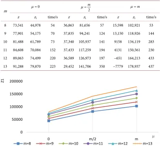
DOI: 10.4236/ojop.2018.74004 76 Open Journal of Optimization Table 3. Numerical experiment results.

m µ =0 2

m

µ = µ=m

z z1 time/s z z1 time/s z z1 time/s

8 73,541 44,978 54 36,863 81,656 57 15,598 102,921 53 9 77,901 54,175 70 37,835 94,241 124 13,150 118,926 144 10 81,488 61,789 73 37,340 105,937 141 9158 134,119 283 11 84,608 70,084 152 37,433 117,259 194 4131 150,561 230 12 89,063 74,499 220 36,589 126,973 197 −651 164,213 433 13 91,288 79,870 223 29,452 141,706 350 −7779 178,937 437

Figure 1. Relationship between performance cost and risk preference of decision maker.

maker, and the vertical axis is the performance cost z1. In the figure, m=8

means that 8 programs are accepted, others and so on.It can be seen from this

figure that in the case of determining the set of the accepted programs, the

per-formance cost increases with the increase of µ_{, namely if the decision maker}

avoids the risk, the performance cost will increase and the performance revenue will reduce. Therefore, decision maker can obtain an ideal performance sche-duling solution based on their own risk preference.

6. Conclusions

This paper studies a problem of uncertain duration performance scheduling un-der accepting strategy, the accepted programs will bring in revenue, and the re-jected programs will produce corresponding penalty cost. After determining the set of the accepted performance programs, the decision maker’s risk preference coefficient is introduced, and the min-max robust performance scheduling model of these accepted programs is built, and then it is transformed into a 0 - 1 mixed linear programming model to minimize the performance cost. Based on this, we combined with the revenue of the accepted programs and the penalty cost of the rejected programs, the algorithm H for solving the performance scheduling problem under accepting strategy is proposed, which provides a ref-erence for decision maker to choose the ideal program scheduling scheme.

0 50000 100000 150000 200000

0 m/2 m

Z1

μ

(13)

This article does not limit the sequence of program performance, but in the actual world, the decision maker will arrange a program at the opening or finale. Or depending on the type of program, some programs must not be adjacent. In addition, multi-objective functions can also be studied, such as maximizing overall revenue on the basis of ensuring that the performance cost does not ex-ceed the budget.

Conflicts of Interest

The authors declare no conflicts of interest regarding the publication of this pa-per.

References

[1] Cheng, T.C.E., Diamond, J.E. and Lin, B.M.T. (1993) Optimal Scheduling in Film Production to Minimize Talent Hold Cost. Journal of Optimization Theory and

Applications, 79, 479-492. https://doi.org/10.1007/BF00940554

[2] Nordström, A.L. and Tufekci, S. (1994) A Genetic Algorithm for the Talent Sche-duling Problem. Computers & Operations Research, 21, 927-940.

https://doi.org/10.1016/0305-0548(94)90021-3

[3] Bomsdorf, F. and Derigs, U. (2008) A Model, Heuristic Procedure and Decision Support System for Solving the Movie Shoot Scheduling Problem. OR Spectrum, 30, 751-772. https://doi.org/10.1007/s00291-007-0103-6

[4] Garcia De La Banda, M., Stuckey, P.J. and Chu, G. (2011) Solving Talent Scheduling with Dynamic Programming. INFORMS Journal on Computing, 23, 120-137. https://doi.org/10.1287/ijoc.1090.0378

[5] Wang, S.Y., Chuang, Y.T. and Lin, B.M.T. (2016) Minimizing Talent Cost and Op-erating Cost in Film Production. Journal of Industrial and Production Engineering, 33, 17-31.

[6] Qin, H., Zhang, Z.Z., Lim, A., et al. (2016) An Enhanced Branch-and-Bound Algo-rithm for the Talent Scheduling Problem. European Journal of Operational

Re-search, 250, 412-426. https://doi.org/10.1016/j.ejor.2015.10.002

[7] Sakulsom, N. and Tharmmaphornphilas, W. (2014) Scheduling a Music Perfor-mance Problem with Unequal Music Piece Length. Computers & Industrial

Engi-neering, 70, 20-30. https://doi.org/10.1016/j.cie.2013.12.017

[8] Zhen, L., Liu, B. and Wang, W.C. (2017) Scheduling of Performance with Mixing Piece Length. Journal of Systems Management, 26, 850-856.

[9] Wang, Y. and Tang, J.F. (2016) A Two-Stage Robust Optimization Method for Solving Surgery Scheduling Problem. Journal of Systems Engineering, 31, 431-440. [10] Xu, X.Q., Cui, W.T., Lin, J. and Qian, Y.J. (2013) Robust Identical Parallel Machines

Scheduling Model Based on Min-Max Regret Criterion. Journal of Systems

Engi-neering, 28, 729-737.

[11] Qiu, R.Z. and Huang X.Y. (2011) A Robust Supply Chain Coordination Model Based on Minimax Regret Criterion. Journal of Systems Management, 20, 296-302. [12] Zhang, L., Chen, T. and Huang, J. (2014) Emergency Network Model and

Algo-rithm Based on Min-Max Regret Robust Optimization. Chinese Journal of

Man-agement Science, 22, 131-139.

(14)

DOI: 10.4236/ojop.2018.74004 78 Open Journal of Optimization 35-53. https://doi.org/10.1287/opre.1030.0065

[14] Bertsimas, D. and Sim, M. (2003) Robust Discrete Optimization and Network Flows.

Mathematical Programming, 98, 49-71. https://doi.org/10.1007/s10107-003-0396-4

[15] Charalambous, C. and Conn, A.R. (1978) An Efficient Method to Solve the Mini-max Problem Directly. SIAM Journal on Numerical Analysis, 15, 162-187.

https://doi.org/10.1137/0715011

[16] Yao, E.Y., He, Y. and Cheng, S.P. (2001) Mathematical Planning and Combination Optimization. Zhejiang University Press, Hangzhou, 31-35.