A Non-Conventional Coloring of the Edges of a Graph
Sándor Szabó
Department of Applied Mathematics, Institute of Mathematics and Informatics, University of Pécs, Pécs, Hungary
Email: [email protected]
Received August 15, 2012; revised September 3, 2012; accepted September 15, 2012
ABSTRACT
Coloring the nodes of a graph is a commonly used technique to speed up clique search algorithms. Coloring the edges of the graph as a preconditioning method can also be used to speed up computations. In this paper we will show that an unconventional coloring scheme of the edges leads to an NP-complete problem when one intends to determine the op- timal number of colors.
Keywords: Maximum Clique; Coloring the Vertices of a Graph; Coloring the Edges of Graph; NP-Complete Problems
1. Introduction
Let be a finite simple graph. This means that has finitely many nodes, that is,
G V,E
G V is finite. Fur-
ther does not have any double edge or loop. In this special case an edge of can be identified with a two element subset of . As a consequence the set of edges of G is a family of two element subsets of . A subgraph of G is called a clique if two distinct nodes of are always adjacent in G. A clique with nodes is simply called a -clique. The number of nodes of a clique is sometimes referred as the size of the clique. A 1-clique inGis a vertex of . A 2-clique in is an edge in . A 3-clique in is sometimes referred as a triangle in . A -clique in is called a maximal clique if it is not a subgraph of any -clique in . A k-clique in is defined to be a maximum clique if
does not contain any G
G G
G
G
k V
k E
G
V
G k
G G
G
G
k
k1
1
-clique. The graph may have several maximum cliques. However, each maximum clique in has the same number of nodes. This well defined number is called the clique size of and it is denoted by .
G
G G
G
Determining the size of a maximum clique in a given graph is an important problem in applied and pure dis- crete mathematics. A number of selected applications are presented in [1] and [2]. It was recognized in [3] that the efficiency of the clique search algorithms can be cru- cially improved by coloring and rearranging the nodes of the tested graph. In [4] instead of coloring the nodes a technique based on dynamic programming was used successfully. In [5] another coloring idea was presented. This time the edges of the graph were colored. Numerical evidence shows that the edge coloring provides sharper upper bounds for the clique size than the node coloring.
However, the improved upper bound comes for a higher computational cost.
We color the nodes of a finite simple graph G
V,E
using colors. We assume that the coloring satisfies the following conditions: 1) Each node of receives ex- actly one color; 2) Adjacent nodes in never receive the same color. We will call this an type coloring of the nodes of withk
G G L
G kcolors. The letter refers to the expression legal coloring. We may use the numbers as colors. The coloring can be defined by a map
L
1, , k
,
: 1,
f v k which is onto. Provided that
v1
v2 ,v1 2f f v
, v v
imply that v1 and v2 are not ad-
jacent for each 1 2V.
We color the edges of a finite simple graph G
V,E
using colors. We suppose that for the coloring the next two conditions hold: 1) Each edge of receives exactly one color; 2) Ifk
G , , ,
x y u v are nodes of a 4-cli-que in G, then the edges
x y,k
and
cannot have the same color. We will call this a type coloring of the edges of with colors. In a conversation Bogdán Zaválnij proposed this edge coloring scheme. The letter comes from the name Bogdán. The color-
, u v B G
B
ing can be described by a map g E:
1, , k
that is onto. We require that g
x y,
g
u v,
, and
x y, u v, imply that x y u v, , ,
, , ,
are not nodes of a 4-clique in G for each
x y u v G E.
Problem 1. Given a finite simple graph and given a positive integer . Decide if the edges of have
type coloring using k colors.
k G
B
The smaller is the number of colors for which the edges of have a type coloring the more useable is the coloring in connection with clique search. The main
k
G B
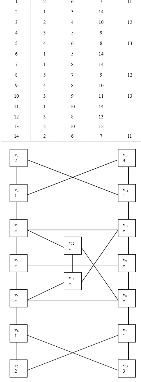
Table 2. The lists of the neighbors of the nodes in H. 3
k . The intuitive meaning of this result is that deter- mining the threshold value of the colors k in Problem 1 is computationally demanding. Consequently, in practical computations we have to resort on approximate greedy algorithms and we have to develop various heuristics.
1 2 6 7
2. The Auxiliary Graph
H
In this section we construct an auxiliary graph. This will play the role of building blocks in further constructions. Let us consider the graph H
V E,
given by its ad- jacency matrix in Table 1. The graph H has 14 nodes1 14 and 24 edges. The rows and columns of the
adjacency matrix of are labeled by the nodes. The bul- let in the cell at the intersection of row i and column
, ,
v v
H
v
j
v records the fact that the unordered pair is an
edge of
,
i j
v v
H . The reader will notice that in Table 1 the node i is replaced by , that is, the letter is sup-pressed and only the index is used. In Table 2 each node and its neighbors are listed. This is another way to describe the graph
v i v
i
H . The set of neighbors of the node in is denoted by and by definition
. Finally, the geometric re- presentation of the graph
v G
N v
N v
V
: ,v x x x E,
His given in Figure 1. Right below each node we recorded the color of the node. But at this moment the reader may ignore the colors. In order to avoid a cluttered figure we used two copies of the nodes 1 and 14. One can imagine that the figure is
drawn on a strip of paper. Then we fold the strip to form a cylinder identifying the shorter sides of the strip. Thus the graph
v v
[image:2.595.56.286.486.737.2]His drawn on the surface of a cylinder and we arrange things such that the two copies of coincide v1
Table 1. The adjacency matrix of graph H.
1 1 1 1 1
1 2 3 4 5 6 7 8 9 0 1 2 3 4
1 × ● ● ● ●
2 ● × ● ●
3 ● × ● ● ●
4 ● × ● ●
5 ● × ● ● ●
6 ● ● × ●
7 ● × ● ●
8 ● ● × ● ●
9 ● ● × ●
1 0 ● ● × ● ●
1 1 ● ● × ●
1 2 ● ● × ●
1 3 ● ● ● ×
1 4 ● ● ● ● ×
11
2 1 3 14
3 2 4 10 12
4 3 5 9
5 4 6 8 13
6 1 5 14
7 1 8 14
8 5 7 9 12
9 4 8 10
10 3 9 11 13
11 1 10 14
12 3 8 13
13 5 10 12
14 2 6 7 11
v1
2
v14
3
v2
1
v11
1
v10
c v3
c
v9
c v4
c
v8
c v5
c
v7
1 v6
1
v14
3 v1
2
v12
c
v13
c
and also the two copies of 14 coincide. The properties
of the graph
v
H we will use later are spelled out for- mally as a proposition.
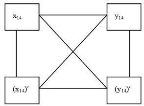
Proposition 1. (1) The graph H does not contain any 3-clique. (2) In an L type coloring of the nodes of H with 3 colors the nodes v1 and 14 must receive the
same color. (3) The nodes of v
H do have an type coloring with 3 colors.
L
Proof. The statements of the proposition can be veri- fied by simple inspections. Here is how the inspection goes in connection with statement (1). Pick the bullet in the cell at the intersection of row and column v2.
This bullet represents the edge
1 2 . Scanning the rows and of the adjacency matrix we can seethat 2 . This means that the edge
1 2 cannot be a side of any triangle in
1
v , v v
1
v N v
2
v
1 N v
v v, H. Thenrepeat the argument for all the 24 edges of H.
In order to prove the statement (2) let us assume on the contrary that there is an L type coloring f V:
1, 2,3
of the nodes of H such that f v
1 f v
143
14f v
. We may
assume that and since this is
only a matter of rearranging the colors 1, 2, 3 among each other. Note that
1 f v 2
1f v and f v
11
f v
must be equal to 1. From this it follows that 3
2,3 and. A similar argument gives that
10 2,3f v
,
6 7
f v f v must be equal to 1 and f v
5 2,3 ,
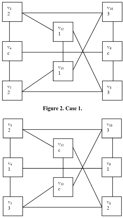
8 2,3 [image:3.595.321.522.83.438.2]f v . This portion of the reasoning can be fol- lowed in Figure 1. We distinguish four cases listed in Table 3. Let us consider case 1. As f v
3 2 and, it follows that
8 2f v f v
12 1 must hold. Simi-larly, must hold. But v12 and 13 are ad- jacent nodes in and so we get the contradiction that
12 13
13f v
1 H
v
f v f
5 3f v
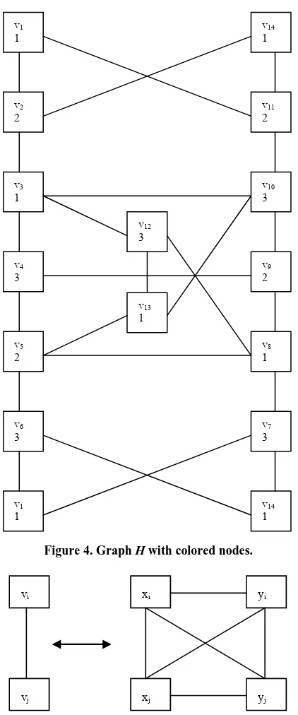
v . The situation is illustrated in Figure 2. Let us consider case 2. From and
, it follows that
3 2f v
4 1f v
v
must hold. Simi- larly, must hold. But 4 and 9 are adja- cent nodes in
9f v 1 v
H and so we get the contradiction that
4
9
f v f v . Each of the remaining cases can be han-dled in an analogous way. The reasoning can be followed in Figure 3.
The statement (3) can be proved by exhibiting a re- quired coloring. This is done in Figure 4.
3. The Auxiliary Graph
K
[image:3.595.56.288.663.735.2]Using the graph H we construct a new graph K. Let
Table 3. The cases.
case f(v3) f(v10) f(v5) f(v8)
1 2 3 2 3 2 2 3 3 2 3 3 2 2 3 4 3 2 3 2
v3
2
v10
3
v4
c
v5
2
v9
c
v8
3 v12
1
v13
1
Figure 2. Case 1.
v3
2
v10
3
v4
1
v5
3
v9
1
v8
2 v12
c
v13
c
Figure 3. Case 2.
1, , 14
x x , 1 14 be pair-wise distinct points. These
will be the nodes of . We connect the nodes , ,
y y
K xi and
i for each
y i, 1 i 14. The edge
x yi, i
of and the node ofK
i
v H correspond to each other mutually. The edges
x yi, i
i, 1 i 14K
form a matching in In other words these edges do not have any common end points and their end points give all the nodes of . We will call these edges of primary edges. We will call all the other edges of secondary edges. If i and
K.
K
v K
j
v are adjacent nodes in H , then we add the following edges to K.
x xi, j
x yi, j
y xi, j
y yi, j
(1)Figure 5 illustrates the construction. If vi and vj
are not adjacent nodes in H, then we do not add any new edge to K. The new graph K has
2 14 28 nodes and
14 24 4 110 edges.To the node vi of H we assigned the edge
x yi, j
of K. To the edge
v vi, j of H we assigned the 4-clique in K whose nodes are x y xi, ,i j,yj. Collapsingthe nodes xi and yj to one point the edges (1) col-
v1
1
v14
1
v2
2
v11
2
v10
3 v3
1
v9
2 v4
3
v8
1 v5
2
v7
3 v6
3
v14
1 v1
1
v12
3
v13
[image:4.595.306.538.72.515.2]1
Figure 4. Graph H with colored nodes.
yj
vi
vj
xi yi
xj
Figure 5. The correspondence between H and K. phic copy of H . We summarize the properties of K we will need later in two propositions.
Proposition 2. (1)
K 4. (2) In each 4-clique in K there are exactly two primary edges.Proof. Clearly, K contains a 4-clique. In order to prove statement (1) it is enough to verify that K does not contain any 5-clique. We assume on the contrary that
K contains a 5-clique. As the primary edges form a matching in K, a 5-clique in K can have only 0, 1, 2 primary edges. The cases are depicted in Figures 6-8,
Figure 6. A 5-clique without primary edge.
Figure 7. A 5-clique with one primary edge.
Figure 8. A 5-clique with two primary edges.
respectively. The primary edges are marked by double lines. Let us suppose first that the 5-clique does not have any primary edge. Then there are 5 primary edges joining to the 5-clique. From this it follows that H must contain a 5-clique. When the 5-clique contains exactly one primary edge, then the graph H must contain a 4-clique. Finally, when the 5-clique contains exactly two primary edges, then H must contain a 3-clique. But by Proposition 1, H does not contain any 3-clique. This contradiction proves statement (1). Statement (2) can be proved using the same technique.
Proposition 3. (1) The edges of have a type coloring with 3 colors. (2) In each such coloring of the edges of the edges
K B
K
x y1, 1
and
x14,y14
must receive the same color. [image:4.595.67.278.82.588.2]of the nodes of H
V E,
. By Proposition 1, such col- oring exists. Using f we can construct a type col-oring of the edges of
B
1, 2,3
:
g F K
W F,
. Wecan achieve this by setting g
x yi, i
to be equal toi
f v . If and vi vj are adjacent nodes in H, then
the nodes , ,x y xi i j,yj
jare nodes of a 4-clique in K. Now f v
i f v and so g
x yi, i
j, j
i, i
g x
y .
The remaining four edges of the 4-clique we color in the following way. Set g x y , g
x yi, j
to beequal to f v
i
and set g
y xi, j
, g
y yi, j
tobe equal to f v
j . A routine inspection shows that the edges of the 4-clique whose nodes are x y xi, ,i j, jB
: 1, 2
g F
1,
y
K K
,3 have a type coloring with 3 colors. (The reader will notice that in fact we used only 2 colors to color the nodes of the 4-clique.) This coloring procedure can be repeated for each 4-clique in which has exactly two primary edges. By Proposition 2, each 4-clique in has exactly two primary edges and so each edge of is colored. Therefore the edges of have a type coloring with 3 colors. This proves statement (1).
B
: 1, 2
K
K
: f V
In order to prove statement (2) let be a type coloring of the edges of K. Using g we can construct an L type coloring
2,3
B
f V
i
,3 of the nodes of H. Simply we set f v f v
i to be equal to g
x yi, j
.4. The Auxiliary Graph
L
Let K
W F,
,
be an isomorphic copy of
K W F
K
such that the sets and W are disjoint. Using and
W K
x14, y14
K
we construct a new graph by adding the following edges to .
L
y14 y
L
14 14
, y , x ,
[image:5.595.98.245.610.719.2]
x14, x14
, ,
14 (2)Figure 9 illustrates the construction. These edges con- nect the graphs and K. The resulting graph is de- noted by L. The graph L has
2 28
56 nodes and
4
2 110 L
224 edges. The properties of the graph we will need later are spelled out in the nextx14
(x14)′
y14
(y14)′
Figure 9. Connecting the graphs K and K′.
proposition.
Proposition 4. (1) The edges of have type col- oring with 3 colors. (2) In such a coloring of the edges of
the edges
L B
L
x y1, 1
and
x14,y14
cannot receive the same color.Proof. By Proposition 3, the edges of K have a type coloring with 3 colors. In such a coloring of the edges of
B
K the edges
x y1, 1
and
x14,y14
must receive the same color. Because the colors of the edges can be exchanged among each other freely we may in fact prescribe the colors of these edges. Similarly, the edges of K have a type coloring with 3 colors. In the coloring of the edges ofB
K the colors of the edges
x1, y1
and
x14 ,
y14
must be equal. Againthe color of these edges can be prescribed. Because of the presence of the edges (2) the edges
x14,y14
and
x14 , y14
must receive distinct colors.5. The Main Result
We are ready to prove the main result of this paper. Theorem 1. Problem 1 is NP-complete for k3. Proof. Let G
V E,
L
be a finite simple graph.
Us-ing we construct a new graph which
satisfies the following two requirements: 1) If the nodes of have an type coloring using 3 colors, then the edges of
G
G
,G V E
G have a type coloring using 3 colors; 2) If the edges of
B
G have a type coloring with 3 col- ors, then the nodes of G have an type coloring with 3 colors.
B
L
Let v1, , vn be all the vertices of G. This means that
1, , vn
i
v
V v . We assign two points i and i to
the node for each
w z
, 1 i i n
i
z
. We choose the points
1 , 1 to be pair-wise distinct. We con-
nect the nodes i and . In other words
, , n
w w z, , n
w z
w zi, i
isan edge of G for each i, 1 i n. For each , , 1
i j i j n we consider an isomorphic copy
, , , ,
i j i j i j
L W F of the auxiliary graph L
W F,
. Ifi
v and vj
G
are adjacent nodes in , then we insert to
G
,
i
L j such that the edge
w zi, i
of G is iden-tified with the edge
xi j, ,1,yi j, ,1
of Li j, . Further theedge
w zj, j
of G is identified with the edge
xi j, ,1 , yi j, ,1
of Li j, . If and vi vj are not adja-
cent in , then we do not add any new node or new edge to
G G.
We may say that the graph is a blown up version of the graph . Each node of is replaced by two connected nodes in
G
G G
One can collapse the nodes wi and of zi G to one point. If
w zi, i
and
w zj, j
are connected with anisomorphic copy i j, of , then one can collapse
to a single edge. In this way one recovers the graph from the graph .
L
G
L Li j,
G
Let us suppose first that the nodes of G
V E,
E . We
3
V,have an type coloring . We define
an edge coloring g: G
set
L
,
i i
1 : , 2,
2,3 of f V
1, E
g w z to be equal to f v
i
. If vi and vje adjacent nodes in G, then in the way we have seen in the proof of Proposition 4 we can extend the coloring of the edges
w zi, i
xi j, ,1,yi j, ,1
andar
h e e graph
Thus the edges of a
tha is a
ty
w zi, i
xi j, ,1 , yi j, ,1
to eac
have
t
dge
: 1
of th
type coloring as
, 2,3
,i j
L .
clai
G B
med in statement (1).
Let us suppose next g E B
pe coloring of the edges of G
V ,
coloringE
. We define a
: 1, 2,3
f V of t G by setting
ihe nodes of
f v to be equal tog
w zi, i
. We claim that
f v and i j at vi and
f vi j imply th vj are
des in In order to pro e the claim let us assume on the contrary that f v
i f v
, i jnot adjacent no G. v
j
and the nodes vi, vj are adjacent in ro
G
, ,
. By P
posi-tion 4, g
xi j, ,1 yi j, ,1
g
xi j, ,1 yi j, ,1
g giv
holds.
On the other hand the definition of t e coloh rin es that
,
,
f vi g w zi i g xi j, ,1 yi, ,1 . Similarly, by the
, ,1
i
j
,1
i
definition of the coloring
m
we get the contradiction
i
i, i
j ,
,j f v g w z g x y
. Fro this
i
jf v f v
ld recall t
graph a . This
o th
nd su proves
the proof on ou e result
th
6. The Derived Graph
ple ppose
pa
From we construct a new graph . The nodes of
G
U F, are the edges of , that is, G UE. Two distinct nodes
x y, and
u v,
of are connected
x y, u v, statement (2).
To complete e sh
at the problem of deciding if the nodes a given simple graph have a L type coloring with 3 colors is an NP- complete problem. Proofs of this well-known result can be found for example in [6,7].
Let G
V E,
be a finite simthat find a B type coloring of the edges of G. A possible interpretation of the main result of this per is that determining the optimal number of colors is a computationally demanding problem. In practical com- putations we should be content with suboptimal values of the number of colors.
we want to
in Γ if and x y u v, , , are not nodes of a 4-clique in . In the lack of established terminal- ogy we call the derived graph of G. The essential con- nection between G and
G
is the following result. Proposition 5. The nodes of have an type col- oring with k colors if and only if the edges of have a
type coloring with k colors.
L
G B
The reader will not have any difficulty to check the veracity of the proposition. The result makes possible to apply all the greedy coloring techniques developed for coloring the nodes of a graph. When the graph has n nodes it may have
G
2O n G
G
edges. For instance when has 4000 nodes, then may have 10 millions edges. In this case the adjacency matrix of does not fit into the memory of an ordinary computer. Thus one should compute the entries of the adjacency matrix from the adjacency matrix of during the coloring algorithm. The most commonly used greedy coloring of the nodes of a graph takes
G
2O n steps. Applying this technique to the derived graph we get an algorithm whose compu-tational complexity is
4O n . The author has carried out a large scale numerical experiment with this algo-rithm. The results are encouraging.
REFERENCES
[1] I. M. Bomze, M. Budinich, P. M. Pardalos and M. Pelillo, “The Maximum Clique Problem,” In: D.-Z. Du and P. M. Pardalos, Eds., Handbook of Combinatorial Optimization, Kluwer Academic Pubisher, Dordrecht, 1999, pp. 1-74. [2] D. Kumlander, “Some Practical Algorithms to Solve the
Maximal Clique Problem,” Ph.D. Thesis, Tallin Univer-sity of Technology,Tallinn, 2005.
[3] R. Carraghan and P. M. Pardalos, “An Exact Algorithm for the Maximum Clique Problem,” Operation Research Letters, Vol. 9, No. 6, 1990, pp. 375-382.
doi:10.1016/0167-6377(90)90057-C
[4] P. R. J. Östergård, “A Fast Algorithm for the Maximum Clique Problem,” Discrete Applied Mathematics, Vol. 120, No. 1-3, 2002, pp. 197-207.
doi:10.1016/S0166-218X(01)00290-6
[5] S. Szabó, “Parallel Algorithms for Finding Cliques in a Graph,” Journal of Physics: Conference Series, Vol. 268, No. 1, 2011, Article ID: 012030.
doi:10.1088/1742-6596/268/1/012030
[6] M. R. Garey and S. Johnson, “Computers and Intractabil- ity: A Guide to the Theory of NP-completeness,” Free- man, New York, 2003.