Journal of Engineering and Applied Sciences 15 (6): 1426-1430, 2020 ISSN: 1816-949X
© Medwell Journals, 2020
Rainfall Analysis of the Makassar City using Thiessen Polygon
Method Based on GIS
1
Sudirman Nganro,
2Slamet Trisutomo,
3Roland A. Barkey and
2Mukti Ali
1Department of Architecture, Faculty of Engineering,
2
Laboratory of Waterfront City, Faculty of Engineering, Hasanuddin University,
92173 Gowa indonesia
3
Laboratory of Planning and Forestry Information System, Faculty of Forestry,
Hasanuddin University, 90245 Makassar, Indonesia
Abstract: Precipitation is the descent of water from the atmosphere to the surface of the earth which is usually rain, snow, fog, dew and hail, the amount of water falling on the surface of the earth can be measured by rain gauges, the distribution of rain in the space can be known by measuring rain in some locations and areas reviewed. In a variety of human activities, rainfall becomes one of the data needs, especially in the study of water availability for consumption, irrigation building planning and mapping of flooded areas. This study aims to analyze local rainfall data on research objects by utilizing global weather data, the observation period for 15 years i.e., from 2000-2014. This research using Thiessen polygon method based on Geographic Information System (GIS) application, rainfall data sourced from global wheater, accessed on August 28, 2017. The results showed that the distribution of rainfall in the research object is represented by 2 rainfall stations, namely station p_521194 and station p_521197. The highest maximum daily rainfall occurred in 2002 of 149.80 mm while the lowest occurred in 2008 amounted to 68.76 mm. Rainfall data will be used to analyze flood discharge in Makassar city.
Key words: Rainfall analysis, Thiessen polygon method, GIS, Makassar city, availability, geographic
INTRODUCTION
Regional rainfall should be estimated from some rainfall observation points. One method of calculating rainfall is the polygon Thiessen method (Singh, 2013; Booij, 2005; El-Khoury et al., 2015; Gibbs et al., 2016), this method takes into account the weight of each station that represents the surrounding area, the Thiessen polygon is fixed for a particular rain station network, if there is a change of rain station network, again a new polygon. Rain is a form of precipitation of water vapor coming from clouds in the atmosphere, rainfall occurs due to evaporation of water, especially water from the surface of the rising sea water into the atmosphere and cools, then distills and falls partly into the sea and partly on land, Water rain falling on the land, partly seeping into the soil (infiltration), partially retained by plants (intercept), partly evaporating and partly moist (Cho, 2016).
Inundated rainfall flows as surface runoff, some falling on the flat surface will form a retention basin while the other leads to a lower area and falls into the channel. The water in the reservoirs, canals and seas will also
undergo evaporation, condensation, so that, it becomes sublimated to rain and fall back, this process is called the hydrologic cycle. Rain can be divided into three types based on the process of precipitation, i.e., convection rain, orographic rain and frontal rain. Rainfall unit measured in mm/inch, 1 mm rainfall means rain water that falls after 1 mm does not flow, not pervasive and does not evaporate. The precipitation required for the preparation of a water use design and flood control design is the average rainfall in the whole area concerned, not rainfall at a particular point, this rainfall is called regional rainfall and is expressed in mm. Sudirman stated that one of the factors that affect the flood/inundation is rainfall.
This study aims to calculate the rainfall of Makassar city region using the Thiessen polygon method based on Geographic Information System (GIS) application.
MATERIALS AND METHODS
Research object: The study is located in the Makassar city of the capital of South Sulawesi province, geographically the city of Makassar lies between
J. Eng. Applied Sci., 15 (6): 1426-1430, 2020
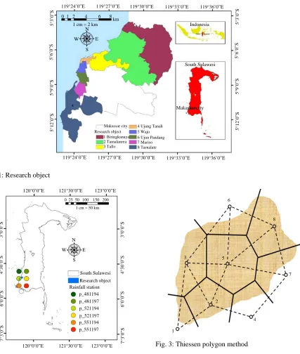
[image:2.612.89.276.356.594.2]Fig. 1: Research object
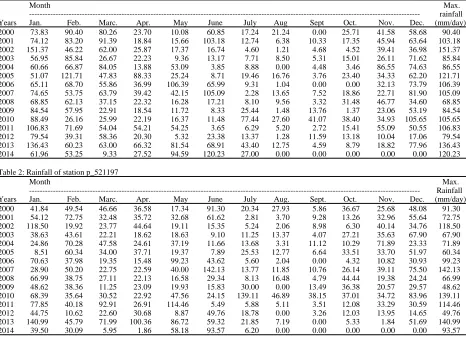
Fig. 2: Rainfall station
119°0’36”-119°32’59” East Longitude (EL) and between 4°54’36”-5°8’19” South Latitude (SL). Research object as shown in Fig. 1.
Research data sources: The data used to calculate rainfall in Makassar city is sourced from http://globalweather.tamu.edu/accessed on August, 28, 2017, precipitation data downloaded from January 1st 2000-July 31th 2014 (15 years) consisting of 6
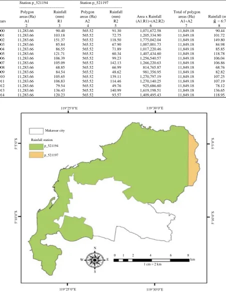
Fig. 3: Thiessen polygon method
observation stations and located at the decimal coordinates -4.8283, 199.7125 North-East corner up to -5.7581, 119.2511 South-West corner. The position of the rainfall station is shown in Fig. 2.
Thiessen polygon method: If the observation points within the area are not evenly distributed, then the mean rainfall calculation is done by taking into account the area of influence of each observation point. On an area within the watershed it is assumed that the rain is the same as that at the nearest station, so that, the recorded rain at a
5°
3’
0”S
5°
6’
0”S
5°
9’
0”S
5°
12
’0”
S
119°24’0”E 119°27’0”E 119°30’0”E 119°33’0”E 119°36’0”E 0 1 2 4 6 8
km 1 cm = 2 km
N
W E
S
Indonesia
South Sulawesi
Makassar city
Makassar city Research object
1 Biringkanaya 2 Tamalanrea 3 Tallo
4 Ujung Tanah 5 Wajo 6 Ujun Pandang 7 Mariso 8 Tarnalate
5°
3’
0”S
5°
6’
0”S
5°
9’
0”S
5°
12
’0”
S
119°24’0”E 119°27’0”E 119°30’0”E 119°33’0”E 119°36’0”E
3°
0’
0”S
4°
30
’0”
S
6°
0’
0”S
7°
3’
0”S
120°0’0”E 121°30’0”E 123°0’0”E
0 25 50 100 150 200
South Sulawesi Research object Rainfall station
p_481194 p_481197 p_521194 p_521197 p_551194 p_551197 N
W E
S
120°0’0”E 121°30’0”E 123°0’0”E
3°
0’
0”S
4°
30
’0”
S
6°
0’
0”S
7°
3’
0”S
1 cm = 50 km
6
5
1 3
2
4
[image:2.612.326.524.361.565.2]J. Eng. Applied Sci., 15 (6): 1426-1430, 2020
station represents that area (Triatmodjo, 2013; Yekti, Permana, 2007; Kawet, Halim, 2013). Rainfall in the area can be calculated by the following Eq. 1:
(1)
A1R1+A2R2+, ..., +AnRn R
A1+A2+, ..., An
Where:
: Rainfall area
R
R1, R2, ..., Rn : Rainfall in each observation point and n is the number of observation points A1, A2, ..., An : The area representing the station 1,
2, 3, ..., n
Figure 3 shows that the area of rain measured by an observation is limited by broken lines.
RESULTS AND DISCUSSION
The rain gauge only provides the depth of rain on which the station is located, so that, rain on an area should be estimated from that point of measurement. Thiessen polygon method is one method that can be used to calculate the average rainfall in an area. This study uses
6 observation points consisting of stations p_481194, p_481197, p_521194, p_521197, p_551194 and p_551197. Based on the results of the analysis, the distribution of rainfall along with its limits are presented in Figure 4 which are grouped by color. The color shows the representation of the rainfall station on the map.
Figure 4 shows the distribution of rainfall at the research location based on Thiessen polygon, from the figure is calculated the area represented by each station that are p_521194 and p_521197. The area is shown in Fig. 5.
The distribution of rainfall in Fig. 4 shows that the station p_521194 represents the polygon in green. The monthly rainfall data as shown in Table 1.
The polygon with the brown color in Fig. 4 is the distribution of rainfall that represents the station p_521197. The rainfall data is shown in Table 2.
By using the Thiessen polygon method in Eq. 1, the rainfall of the research object can be analyzed, as informed in Table 3.
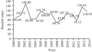
Based on the results of the analysis in Table 3, it can be described graph of rainfall research object as shown in Fig. 6.
Table 1: Rainfall of station p_521194
Month Max.
[image:3.612.74.540.384.721.2]--- rainfall Years Jan. Feb. Marc. Apr. May June July Aug Sept Oct. Nov. Dec. (mm/day) 2000 73.83 90.40 80.26 23.70 10.08 60.85 17.24 21.24 0.00 25.71 41.58 58.68 90.40 2001 74.12 83.20 91.39 18.84 15.66 103.18 12.74 6.38 10.33 17.35 45.94 63.64 103.18 2002 151.37 46.22 62.00 25.87 17.37 16.74 4.60 1.21 4.68 4.52 39.41 36.98 151.37 2003 56.95 85.84 26.67 22.23 9.36 13.17 7.71 8.50 5.31 15.01 26.11 71.62 85.84 2004 60.66 66.87 84.05 13.88 53.09 3.85 8.88 0.00 4.48 3.46 86.55 74.63 86.55 2005 51.07 121.71 47.83 88.33 25.24 8.71 19.46 16.76 3.76 23.40 34.33 62.20 121.71 2006 65.11 68.70 55.86 36.99 106.39 65.99 9.31 1.04 0.00 0.00 32.13 73.79 106.39 2007 74.65 53.75 63.79 39.42 42.15 105.09 2.28 13.65 7.52 18.86 22.71 81.90 105.09 2008 68.85 62.13 37.15 22.32 16.28 17.21 8.10 9.56 3.32 31.48 46.77 34.60 68.85 2009 84.54 57.95 22.91 18.54 11.72 8.33 25.44 1.48 13.76 1.37 23.06 53.19 84.54 2010 88.49 26.16 25.99 22.19 16.37 11.48 77.44 27.60 41.07 38.40 34.93 105.65 105.65 2011 106.83 71.69 54.04 54.21 54.25 3.65 6.29 5.20 2.72 15.41 55.09 50.55 106.83 2012 79.54 39.31 58.36 20.30 5.32 23.38 13.37 1.28 11.59 13.18 10.04 17.06 79.54 2013 136.43 60.23 63.00 66.32 81.54 68.91 43.40 12.75 4.59 8.79 18.82 77.96 136.43 2014 61.96 53.25 9.33 27.52 94.59 120.23 27.00 0.00 0.00 0.00 0.00 0.00 120.23
Table 2: Rainfall of station p_521197
Month Max.
J. Eng. Applied Sci., 15 (6): 1426-1430, 2020
Table 3: Rainfall analysis using thiessen polygon method
Station p_521194 Station p_521197 ---
Polygon Rainfall Polygon Rainfall Total of polygon
areas (Ha) (mm) areas (Ha) (mm) Area x Rainfall areas (Ha) Rainfall (mm) Years A1 R1 A2 R2 (A1.R1)+(A2.R2) A1+A2 Rˆ = 6:7 1 2 3 4 5 6 7 8
2000 11,283.66 90.40 565.52 91.30 1,071,672.58 11,849.18 90.44
2001 11,283.66 103.18 565.52 72.75 1,205,334.90 11,849.18 101.72
2002 11,283.66 151.37 565.52 118.50 1,775,042.04 11,849.18 149.80
2003 11,283.66 85.84 565.52 67.90 1,007,001.73 11,849.18 84.98
2004 11,283.66 86.55 565.52 71.89 1,017,220.46 11,849.18 85.85
2005 11,283.66 121.71 565.52 60.34 1,407,434.60 11,849.18 118.78
2006 11,283.66 106.39 565.52 99.23 1,256,540.57 11,849.18 106.04
2007 11,283.66 105.09 565.52 142.13 1,266,220.63 11,849.18 106.86
2008 11,283.66 68.85 565.52 66.99 814,765.87 11,849.18 68.76
2009 11,283.66 84.54 565.52 48.62 981,356.95 11,849.18 82.82
2010 11,283.66 105.65 565.52 139.11 1,270,797.19 11,849.18 107.25
2011 11,283.66 106.83 565.52 114.46 1,270,140.25 11,849.18 107.19
2012 11,283.66 79.54 565.52 49.76 925,686.60 11,849.18 78.12
2013 11,283.66 136.43 565.52 140.99 1,619,198.51 11,849.18 136.65
2014 11,283.66 120.23 565.52 93.57 1,409,495.43 11,849.18 118.95
Fig. 4: Rainfall distribution based on research object
119°25’0”E 119°30’0”E
5°
5’
0”S
5°
10
’0”
S
5°
5’
0”S
5°
10
’0”
S
119°25’0”E 119°30’0”E
0 1 2 4 6 8
1 cm = 2 km
km N
W E
S Makassar city
Rainfall station
p_521194
J. Eng. Applied Sci., 15 (6): 1426-1430, 2020
160 140 120 100 80 60 40 20 0
149.80
101.72
90.44
118.78
84.98 85.85 106.04
06.86
68.76 82.82
107.25 107.19
78.12 136.65
118.95
R
a
in
fa
ll
(
m
m
)
200
2
20
00
20
0
1
20
0
3
20
0
4
20
05
20
0
6
20
0
7
20
0
8
20
0
9
20
1
0
20
1
1
20
1
2
20
13
20
14
[image:5.612.67.255.100.214.2]Yrars
Fig. 5: The area that represents the station
Fig. 6: Rainfall chart of the research object CONCLUSION
A period of observation for 15 years, i.e., from 2000-2014. The results show that the distribution of rainfall is grouped into 2 polygons each representing stations p_521194 and p_521197. Based on the results of
the analysis, the data show that the highest rainfall occurred in 2002 which amounted to 149.80 mm while rainfall the lowest occurrence in 2008 of 68.76 mm.
ACKNOWLEDGEMENT
The researchers would like to thank ESRI Indonesia for providing ArcGis 10.5 Software to support the implementation of this research.
REFERENCES
Booij, M.J., 2005. Impact of climate change on river flooding assessed with different spatial model resolutions. J. Hydrol., 303: 176-198.
Cho, S.E., 2016. Stability analysis of unsaturated soil slopes considering water-air flow caused by rainfall infiltration. Eng. Geol., 211: 184-197.
El-Khoury, A., O. Seidou, D.R. Lapen, Z. Que, M. Mohammadian, M. Sunohara and D. Bahram, 2015. Combined impacts of future climate and land use changes on discharge, Nitrogen and Phosphorus loads for a Canadian river Basin. J. Environ. Manage., 151: 76-86.
Gibbs, M.S., K. Clarke and B. Taylor, 2016. Linking spatial inundation indicators and hydrological modelling to improve assessment of inundation extent. Ecol. Indic., 60: 1298-1308.
Singh, B.R., 2013. Climate Change: Realities, Impacts Over Ice Cap, Sea Level and Risks. IntechOpen, Rijeka, Croatia, ISBN: 978-953-51-0934-1, Pages: 508.
12,000
10,000
8,000
6,000
4,000
2,000
p_521194 p_521197 Areas (Ha)
Va
lue
[image:5.612.85.275.260.369.2]