warwick.ac.uk/lib-publications
Original citation:
Kiselychnyk, Oleh, Bodson, Marc and Wang, Jihong. (2015) Linearized state-space model of a
self-excited induction generator suitable for the design of voltage controllers. IEEE
Transactions on Energy Conversion, 30 (4). pp. 1310-1320
.Permanent WRAP URL:
http://wrap.warwick.ac.uk/78812
Copyright and reuse:
The Warwick Research Archive Portal (WRAP) makes this work by researchers of the
University of Warwick available open access under the following conditions. Copyright ©
and all moral rights to the version of the paper presented here belong to the individual
author(s) and/or other copyright owners. To the extent reasonable and practicable the
material made available in WRAP has been checked for eligibility before being made
available.
Copies of full items can be used for personal research or study, educational, or not-for profit
purposes without prior permission or charge. Provided that the authors, title and full
bibliographic details are credited, a hyperlink and/or URL is given for the original metadata
page and the content is not changed in any way.
Publisher’s statement:
“© 2015 IEEE. Personal use of this material is permitted. Permission from IEEE must be
obtained for all other uses, in any current or future media, including reprinting
/republishing this material for advertising or promotional purposes, creating new collective
works, for resale or redistribution to servers or lists, or reuse of any copyrighted component
of this work in other works.”
A note on versions:
The version presented here may differ from the published version or, version of record, if
you wish to cite this item you are advised to consult the publisher’s version. Please see the
‘permanent WRAP url’ above for details on accessing the published version and note that
access may require a subscription.
Abstract— The complexity and strong nonlinearity of the model of a self-excited induction generator hinders the systematic design of a voltage regulation system. Using a special reference frame aligned with the stator voltage vector, the paper succeeds in developing a control-oriented linearized model that relates small deviations of the capacitance, load admittance, and angular velocity, to corresponding deviations of the voltage amplitude. Transfer functions are also computed based on the linear model. A stability analysis predicts rapidly-decaying oscillatory transients combined with a primary component with slower exponential decay. Simulated transient responses of the full and linearized models demonstrate the validity of the approximation and are in good agreement with experiments.
Index Terms—induction generator, self-excitation, linearized dynamic model, renewable energy, electric machines.
I. INTRODUCTION
elf-excited induction generators (SEIG) have found applications in renewable energy (wind and hydro) for the off-grid production of power. The main advantage of SEIGs compared to synchronous generators is that they are relatively inexpensive and possess natural short-circuit protection properties. They are used for feeding pumps, heating and lighting systems, and as portable generators.
One of the problems of power generation based on SEIG’s is the voltage fluctuations caused by load changes or angular velocity disturbances, restricting the types of possible loads. Researchers have proposed a number of solutions for voltage stabilization [1]-[2], based on electronic converters. They include controlled inductors, capacitors, and dump loads, which are generally referred to as electronic load controllers. Other solutions are based on voltage or current source inverters using a DC bus (also referred to as generalized impedance controllers), and static synchronous compensators.
Manuscript received June 10, 2014.
This work was supported in part by Advantage West Midlands and the European Regional Development Fund, funders of the Science City Research Alliance Energy Efficiency Project – a collaboration between the Universities of Birmingham and Warwick.
O. Kiselychnyk and J. Wang are with the School of Engineering, University of Warwick, Coventry, CV4 7AL, UK (e-mails:
[email protected], [email protected])
M. Bodson is with the ECE Department, University of Utah, Salt Lake City, UT 84112, USA (e-mail: [email protected])
In all cases, the control task is to stabilize the voltage at the output of the SEIG. In some of the systems, internal control loops are implemented for stator currents [3]-[6], load currents [7], and AC input/output currents of the converters [4], [8]-[10] to make them current sources. Since the model of the SEIG is nonlinear and of high order (upwards from sixth order for purely resistive loads), the problem of systematic control design is very complicated. Therefore, typical control structures have been applied with P or PI voltage controllers whose parameters are chosen heuristically and iteratively based on simulations or experiments.
In terms of control methodologies, a sliding mode voltage controller is designed in [11]. It is obtained for the SEIG with linear magnetics based on a model in stator coordinates. Space vector voltage control in an arbitrary rotating reference frame is developed in [12] based on a root locus approach and a linearized model obtained neglecting the nonlinearity of the magnetizing inductance. Validation is only provided through simulations in [11] and [12].
A control system is implemented in [3] in a synchronous reference frame with four PI-controllers for voltage, frequency, and stator currents. The authors indicate that they are unaware of a proven systematic approach for control design or a suitable small-signal linearized model. The present paper aims to remedy this situation.
An interesting solution is proposed in [4], where the choice of reference frame allows the decoupling of frequency and voltages in steady-state. The method utilizes a steady-state SEIG model derived from the nonlinear model in the synchronous reference frame, but does not use it to control the dynamics of the system.
Direct voltage control is developed in [13], resulting in a PI voltage controller, a lead-lag compensator to increase stability margins, and a feedforward compensator for voltage harmonics. However, the results are obtained through a linearization of the SEIG model and do not account for magnetic saturation (the magnetizing inductance is assumed constant). The model is multi-input multi-output and is transformed into single-input single-output systems by considering cross-coupling terms as disturbances.
A DC bus voltage controller is obtained in [14] based on input-output linearization applied to the model of the SEIG with inverter considering a constant magnetizing inductance. A sliding mode DC bus voltage controller is also designed. A
Linearized State-Space
Model of a Self-Excited
Induction Generator Suitable for the Design of
Voltage Controllers
Oleh Kiselychnyk,
Member, IEEE
, Marc Bodson,
Fellow, IEEE,
and Jihong Wang,
Senior Member,
IEEE
linear optimal controller is obtained for SEIG regulation through a static synchronous compensator in [9] based on augmented state equations derived from the model of the SEIG with the fluxes as state variables, but without accounting for magnetic saturation. The control law is implemented in the reference frame aligned with the load voltage vector.
A linearized model of the SEIG is obtained in [15] by applying a Taylor’s expansion. However, the model is obtained from the simplified nonlinear SEIG model neglecting the time derivative of the magnetizing inductance (cross-saturation effect) and ignoring additional terms in the linearized model. Such an approach is only correct for analyzing the system behavior around the zero steady state (self-excitation onset), but is questionable otherwise [15], [16]. In [17], a linearized SEIG model is developed for the case of the SEIG feeding an induction motor and provides useful insights into the dynamics of the system. However, it is not control-oriented and, like [15], describes a way of linearization, rather than an explicit model. A linearized model accounting cross-saturation effect is derived systematically in [18] and the stability of the operating points of the SEIG is assessed through computations of the eigenvalues.
The objective of the present paper is to go beyond the previous analyses by developing a control- oriented linearized state-space model of the SEIG with capacitance, load admittance, and angular velocity perturbations as inputs to the system, and with voltage magnitude as an output. The derivation of the model is difficult, given the complexity of the strongly non-linear model of the SEIG, and it cannot be achieved through standard approaches of linearization theory. However, a solution can be reached by a specific alignment of the reference frame. The derived fifth-order transfer functions are validated through comparison of the simulated voltage transients of the linearized model with the transients of the nonlinear system as well as with experimental data.
The paper is based on results presented earlier by the authors in [19]. The contributions of the present paper expand beyond the previous results by considering input actions such as load admittance and angular velocity, in addition to capacitance. Results are given using a different motor, providing additional validation of the model. Further, the validity is more clearly demonstrated by computing the instantaneous magnitude of the voltage vector based on measurements of the voltages of all three phases (in [19], only one phase voltage was measured). Simulations are also more carefully compared to experiments by applying the measured angular velocity in the simulations.
II. MATHEMATICAL MODEL OF SEIG
A. Nonlinear Model of SEIG
Consider a two-phase model of the induction generator with capacitors and resistive loads connected in parallel with the stator windings. Each phase of the generator is assumed to contain a controllable, variable-capacitor and a variable load resistor. The variable capacitor can be obtained by engaging
parallel capacitors through switching devices (relay, thyristor, or transistor switches), or through chopping of the current in a fixed capacitor. The variable resistor can also be obtained through an electronic load controller by engaging a dump resistor in parallel with the load.
The state-space model of the SEIG accounting for cross-saturation effect in a rotating reference frame was derived in [18] following the unified approach to modeling of induction machines with magnetic saturation from [20]
EXFX, (1)
whereX
USF iSF iRF USG iSG iRG
T,1 2
2 1
F F
F
F F
, F FG
FG G
E E
E
E E
, 1
1 0
1 0
0 0
L S
R
Y
F R
R
,
2
0 0
0 ( )
0 ( )
e
e S M e M
p e M p e R M
C
F L L L
n L n L L
,
0 0
0 0
F S MF MF
MF R MF
C
E L L L
L L L
,
0 0 0
0 0
FG MFG MFG MFG MFG
E L L
L L
,
0 0
0 0
G S MG MG
MG R MG
C
E L L L
L L L
.
In the model, e is the arbitrary angular velocity of an F-G
reference frame with respect to the stator frame, USF, USG,
SF
i , iSG are the F and G components of the stator voltages and currents, respectively, iRF, iRG denote the components of the
rotor currents, YL1/RL is the admittance of the resistive
load (per phase), C is the value of the capacitor (also per phase), is the angular velocity of the rotor, RS and RR are
the stator and rotor resistances, LS and LR denote the stator
and rotor leakage inductances, and np is the number of pole
pairs.
The magnetizing inductance LM f i(M) is a static
function of the magnitude of the magnetizing current
2 2
M MF MG
i i i , (2)
where iMFiSFiRF and iMGiSGiRG. The model is based
on the generalized two-phase model of an induction machine with a choice of stator and rotor currents as state variables. The differentiation of the product of the magnetizing inductance and the magnetizing current with respect to time introduces in the model the nonlinear inductances LMF, LMG
and LMFG [18], where
2 2
( ) /
MF M M MF M
L L LL i i , LMGLM(LLM)iMG2 /iM2 ,
2
( ) /
MFG M MF MG M
L LL i i i , (3)
and LLMi dLM M/diM denotes the dynamic magnetizing
B. Conditions for Self-Excitation
Sustained self-excitation corresponds to the existence of a nonzero steady-state vector X* such that
* * 0
F X , (4)
where *
F is the function F evaluated at the frequency *
e
and *
M
L corresponding to X*. The special structure of the
matrix F allows one to transform the steady-state equation (4) into a complex form
* *
*1 2 0
F jF Z , (5)
where * * *
1 2
Z X jX , * * * 1 2
T
X X X . For (5) to have a
non-zero solution, one needs
* *
1 2
det(F jF )0. (6)
After simple manipulations, the real and imaginary parts of (6) give two equations from the original equation (4) [18]. The first is a polynomial of fifth order in *
e
, with coefficients depending on the generator parameters and operating conditions. The (typically single) real root of the polynomial gives the reference frame angular velocity *
e
(also the generated frequency) associated with a constant state *
X . The second equation is an explicit formula giving *
M
L as a function
of *
e
. For a typical magnetizing inductance curve [18], there can be up to two values of i*M for a given L*M, in general.
The stator voltage amplitude is derived from (5) accounting for (2) evaluated at X* [18]
* * * *
*2 2 *2 2
(1 ) ( )
e M M S
L S e s e L s S
L i U
Y R C L Y L CR
. (7)
The angle of the stator voltage vector is not uniquely defined (self-excitation can occur for any value of phase of the generated voltages). The other state variables are easily obtained from (5) based on (7) choosing an arbitrary angle of the voltage vector.
C. Stability of Self-Excitation
Rotation of the reference frame at the frequency e* transforms
the limit cycles of self-excitation in the stator frame into constant state vectors X*. The stability analysis of these equilibria was performed in [18] based on linearization of the nonlinear differential (matrix) equation (1) and computation of the corresponding eigenvalues. For realistic generator parameters, the following properties of the six eigenvalues were always observed. Four of them were couples of complex conjugates with negative real parts, one was real, and one was equal to zero.
The complex eigenvalues were found to be significantly further in the left-half plane than the fifth real eigenvalue in the vicinity of the corresponding self-excitation boundary, which is typically the realistic operating condition. The fifth eigenvalue was negative when there was a possible solution of
*
M
i belonging to the descending part of the LM curve. The
zero eigenvalue indicated neutral stability of the system and
was associated with the lack of synchronization mechanism in the SEIG: any phase shift of the voltages and currents remains indefinitely.
D. Linearized Model with Capacitance, Load Admittance, and Angular Velocity as Inputs
The magnitude of the SEIG voltages depends on all the parameters including the rotational speed, the load resistance, and the capacitance. The paper considers the case where the capacitance or a part of the load admittance are control variables, whereas other variables are disturbances. The objective of the research is to derive a linearized model (and therefore, transfer functions) considering small independent perturbations of capacitance C, load admittance YL, and
angular velocity as inputs, and the voltage magnitude
perturbation US as output. Such a model could be suitable
for systematic SEIG control design.
The derivation of the model presents several challenges, including:
The relationship between voltage and capacitance, load admittance, and angular velocity is highly nonlinear both for steady-state and dynamic responses. Besides magnetic saturation, a major problem is that the output variable, which is the peak voltage US , is related nonlinearly to the
state variables through 2 2
S SF SG
U U U .
The capacitance and load admittance are parameters of the system rather than external inputs.
Variations of capacitance, load admittance, or angular velocity cause a variation in the frequency *
e
, which is another parameter of the model. It was found that not accounting for this effect could result in an unstable linearized system (even when the nonlinear system was stable).
The region of validity of a linearized model is bounded by the region of operation (i.e, self-excitation) of the system.
These features make the problem unusual, and not fitting the usual framework of linearization theory. Interestingly, the neutral stability of the system is exploited here to resolve the
problem associated with the nonlinearity 2 2
S SF SG
U U U .
In the process, one of the variables is eliminated and a system of reduced order (equal to 5) is obtained.
To develop the technique, consider an equilibrium state X* and perturbations C, YL, and causing perturbations of
the vector X
USF iSF iRF USG iSG iRG
T, andsimultaneous perturbations of the frequency e and of the
inductances LM, LMF, LMG, LMFG. Substitution of the
perturbed variables into system (1) yields
*
*
E X X F X X , (8)
where E is E computed for CC, L*MFLMF,
*
MG MG
L L , *
MFG MFG
C C, YLYL, , *
e e
, *
M M
L L . Subtracting
(4) from (8), using X* 0, and neglecting second-order perturbations, gives the linearized description of the SEIG
* * * *
* * *
,
LM M YL L
C e e
E X F X F L F Y
F C F F
(9)
where * * * 0 0 0 0 SF YL SG U F U , * * * * * 0 0 0 0 e SG C e SF U F U , * * * * * * * * * * * * * * * * * * * ( ) ( ) ( ) ( ) SG S M SG M RG M SG R M RG e
SF
S M SF M RF M SF R M RF
CU
L L i L i
L i L L i
F
CU
L L i L i
L i L L i
* * * * * * * * * 0 ( ) 0 ( ) e MG e p MG LM
e MF p e MF
i n i F i n i , * * * * * * * * * 0 0 ( ) 0 0 ( )
p M SG p R M RG
p M SF p R M RF n L i n L L i F
n L i n L L i
.
The perturbation LM is found from the definition of the
dynamic magnetizing inductance in (3) evaluated at X*. Necessary for its computation is the perturbation iM, which
is derived as a total differential from (2) [19]. Then, the term *
LM M
F L in equation (9) can be transformed to
* *
LM M
F L F X, (10)
where * * * * * * * * * * * * * * * * * * * * 0 ( ) 0 0 0 ( ) e MG MG MG
M e p MG MF MF
M M M M M
e MF p e MF
i
i i
L L n i i i
F
i i i i i
i n i ,
and the linearized model of the SEIG is
* * * *
* * * .
YL L
C e e
E X F F X F Y
F C F F
(11)
Note that the perturbations C, YL and are
independent of each other, while e depends on all of them.
Computation of the perturbation e is possible in the
coordinate frame aligned with the stator voltage vector at all times (which is possible since steady-state phase is not
uniquely defined). Thus, USF* US* , USG* 0, USF US ,
and USG0. With d(USG) /dt0, the fourth differential
equation in (11) transforms into an algebraic equation
* *
e FeX X FeC C
, (12)
where
* *
* * *
1
0 0 0
| | | | | |
e L
eX
S S S
Y F
U C U C U
, and
* *
/
eC e
F C.
The linearized model of the SEIG in the reference frame aligned with the stator voltage vector is then obtained as
* * * * * *
* * * *
( ) .
e eX YL L
C e eC
E X F F F F X F Y
F F F C F
(13)
The stability properties of system (13) are determined by computation of the eigenvalues of
1
* * * * * *
e eX A E F F F F
. (14)
The matrix A* has dimension 6x6, but its fourth row is zero (and corresponds to the zero eigenvalue). The fourth row and column can thus be dropped, yielding a system with a reduced
state X US iSF iRF iSG iRGT. Then, the
reduced-order state-space representation is defined by
* * * * * , T F FG T FG G
E E W
E
WE WE W
*
* 1 2
*
2 1
,
T T
F F W
F
WF WFW
0 1 0 ,
0 0 1 W
* * * * * * * * * * * * * * * * * * * * 0
( ) 0
( )
e MG
MG MG
M MF MF
e p MG
M M M M M
e MF p e MF
i
i i
L L n i i i
F
i i i i i i
n i ,(15)
and *
C
F , *
e
F , *T eX
F , *
YL
F , F*
remain, but with the fourth row
dropped.
The transfer functions of the system from C, YL, and
to the first element of the state vector are P sC( ), the
“plant” of a voltage regulator with capacitance as a control variable, PYL( )s , the “plant” of a voltage regulator with load
adjustment (or the transfer function from the load disturbance otherwise), and P s( ), the response to an angular velocity
disturbance (see Fig. 1).
PC(s)
Pω(s)
C
ω
YL
|US|
[image:5.612.49.298.92.285.2]PYL (s)
Fig. 1. Block diagram of the control-oriented model of the SEIG.
The internal state that was dropped is associated with the phase of the generated voltages and currents, and does not affect the response from C, YL or to US . The
eigenvalues are the same as those of the original system, except for the zero eigenvalue that was eliminated.
The model in Fig. 1 can be used for the systematic design of voltage controllers. The model is only valid for limited perturbations, and any control input or disturbance perturbation brings the system to another operating point, altering the parameters of the transfer functions.
boundary, the linearized model (13) will predict a stable steady-state, although the nonlinear system will not have a stable operating mode. Therefore, some restrictions must be imposed on the values of the perturbations. In the results presented below, it was checked that the initial and final operating points corresponded to stable self-excitation.
III. COMPUTATIONS AND EXPERIMENTAL RESULTS
A. Experimental Testbed
This section presents the results of experiments and simulations designed to validate the linearized control-oriented model in the reference frame aligned with the stator voltage vector. A three-phase induction motor (Bk2208, with rated values 250 W, 240 V (∆), 50 Hz, and 1425 rpm) was used for experiments as SEIG. The following parameters of the generator were determined experimentally RS=31.65 Ω,
R
R =28.1 Ω, LS LR=0.0921 H, np=2. The analytic
approximation of the magnetizing inductance is given in the appendix.
The SEIG was coupled to another induction motor (M3AA090LB-4, with rated values 1.1 kW, 230 V (∆), 50 Hz, and 1435 rpm) controlled through the frequency converter ABB ACS355 with rated power 1.1 kW feeding the stator windings. The higher value of the motor’s power and the slip compensation function of the ACS355 provided some angular velocity stabilization during experiments.
Voltages were measured in the testbed as line-to-line voltages. Computational values obtained from the analysis of Section II were converted using a Y to ∆ transformation to obtain line-to-line stator voltages. The excitation capacitors and the loads were Y-connected, and the values of load admittances and capacitances shown in the figures are actual values (i.e., line to neutral).
The capacitor bank consisted of nine three-phase capacitors. Eight of them were engaged through three-phase relays controlled through dSPACE DS1104 logical outputs and transistors switches. Additional circuits were implemented to discharge the capacitors after disengaging. The load bank included six three-phase resistors controlled manually through
two-pole toggle switches. The line-to-line voltage
measurements were taken between all three phases through Hall effect voltage transducers LV25-P and read through DS1104 analog-to-digital converters. The angular velocity of the motor was monitored through an A2108 optical tachoprobe.
B. Steady-State Voltage Magnitude Characteristics
Computed and experimental steady-state values of the
line-to-line voltage magnitude USL* , as functions of the capacitance,
are in good agreement and shown for different angular velocities and loads in Fig. 2. A similar accuracy was obtained for the steady-state voltages as functions of angular velocity (in the range from 150 rad/s to 190 rad/s) for C=19 µF, no load, 423 Ω and 523 Ω load resistance cases, and as functions
of load admittance (from no load up to 1/423 1) for the cases of C=19 µF, 21 µF, 31 µF at 160.14 rad/s angular velocity. The relative steady-state error does not exceed 3%.
Note that the voltages reach values significantly higher than the rated peak voltage of 339V. The wide range was chosen to demonstrate the validity of the model. However, only the lower values of capacitors would be used in practice, and were used for transient experiments.
18 20 22 24 26 28 30 32
250 300 350 400 450 500 550 600 650
C, µF Computed
Experimental
ω= 160.14 rad/s No load
423 Ω load 523 Ω load
423 Ω load
ω= 172.7 rad/s |USL * |, V
Fig. 2. Steady-state line-to-line voltage magnitude as a function of capacitance for different angular velocities and loads.
C. Computation of Eigenvalues
The eigenvalues of the matrix A* were computed according to (14) for 160.14rad/s and YL 1/ 423Ω-1 within the
corresponding self-excitation boundary. The complex
eigenvalues were well into the stable side of the plane and the absolute values of their imaginary parts decreased monotonously with increasing capacitance. The main factor influencing the stability was therefore the real non-zero eigenvalue (referred to as #5), which was much closer to the imaginary axis for excitation conditions close to the boundary. The zero eigenvalue had no influence on the dynamics when considering the voltage magnitude as the output.
Fig. 3 shows the possible solutions *
M
i and their associated
eigenvalue #5 over the range of capacitance. The smaller current corresponds to the ascending part of the LM f i(M)
curve (see Appendix) and the larger current corresponds to the descending part. In the region between about 31.5 and 396 µF, only the descending part yields a solution. All operating points of the SEIG belonging to the descending part are found to be stable.
In the typical SEIG operation close to the self-excitation boundary, the computations of the eigenvalues through the ranges of angular velocity (for C=19 µF and YL 1/ 423Ω-1)
and of load admittance (for C=19 µF and 160.14rad/s) have also shown the dominating influence of the eigenvalue 5 on the transient behavior of the system.
The eigenvalues of the model using a fixed LLM were
[image:6.612.323.557.154.315.2]saturation region (such as is sometimes used in the literature) will fail to predict the stability of the self-excited operating mode.
0 100 200 300 400 500
-40 -30 -20 -10 0 10 20 30 40 50 60
C, μF YL =1/423 Ω-1 ω=160.14 rad/s
10iM , * A
Eigenvalues 5 ascending part
descending part
100iM , * A
100iM , * A
0.1·Eigenvalues 5 descending part
ascending part ascending
[image:7.612.60.285.90.256.2]part
Fig. 3. Eigenvalue #5 and magnetizing current as functions of capacitance.
D. Transient Responses
The transient responses *
| | | | | |
USL USL USL of the linearized system are shown in Fig. 4 (a) for a step disturbance
=3.14 rad/s starting at t=5s. The figure also shows the corresponding experimental curve and transients computed for the nonlinear system (1)-(3) in the stationary stator reference frame A-B. Additional results are presented in Fig. 4 (b) both for the linearized and nonlinear models accounting for angular velocity changes starting at t=5s through incorporation of the measured velocity (Fig. 4 (c)) in the simulations. One finds that simulations based on the continuously varying angular velocity, obtained from measurement, are more accurate than those that assume a step change in rotational speed. The responses for step disturbances
C=2 µF,
C=-2 µF, andL
R
=100 Ω, and starting at t=5s are presented in Figs. 5-7 respectively, and compared to the experiments. The measured rotational speed was used in all simulations. The initial operation started with =160.14 rad/s, C=19 µF, and
L
R =423Ω, which was chosen because it provided an SEIG
operating point where the voltage and frequency were close to their rated values.
The transient behavior of the linearized model is very close to the nonlinear model, and is in a good agreement with the experiments. The transient responses fit the prediction of computed eigenvalues, with rapidly decaying oscillations appearing together with a slow exponential decay. Accounting for angular velocity variations in simulations correctly predicts the time and value of the initial overshoot (Fig. 4 (b)), and the small natural oscillations superimposed on the exponential decay (Figs. 4-7). In the case of Figs. 5-7, oscillations originate from oscillations in the angular velocity data in addition to the effect of variations of C and YL. Note that the
angular velocity temporary decreases (Fig. 5) or increases (Fig. 6) from its steady-state value as a result of the torque change, with the slip compensation system eventually restoring the value of velocity.
The large steady-state error between the linearized and nonlinear models in Figs. 5 and 6 is due to the strongly nonlinear behavior of the system that one is attempting to control. A reduction of the magnitude disturbance by a factor of ten makes the error negligible (Fig. 8). Note that, in the case of Fig. 5, the initial negative experimental voltage peak is bigger than simulated one. This feature is due to the fact that the model does not account for the difference between the initial capacitor voltage and the stator voltage. There is no such problem for the case of disengaging of the capacitor (Fig. 6).
5 5.1 5.2 5.3 5.4 5.5
160 161 162 163 164
4.9 5 5.1 5.2 5.3 5.4 5.5
-5 0 5 10 15 20 25 30 35
4.9 5 5.1 5.2 5.3 5.4 5.5
-5 0 5 10 15 20 25 30 35
C=19 μF
YL =1/423 Ω-1
ω=160.14 rad/s Nonlinear
A-B model
t, s Experiment
δω=3.14 rad/s
|USL|, V
Linearized model
Step response simulation
Step response simulation accounting experimental ω
ω, rad/s
t, s Experiment
t, s Experiment
Linearized model
Nonlinear A-B model
|USL|, V
C=19 μF
YL =1/423 Ω-1
ω=160.14 rad/s (a)
(b)
(c)
Fig. 4. Voltage perturbations caused by = 3.14 rad/s: (a) Step response simulations and experiment. (b) Simulations accounting for experimental angular velocity. (c) Measured angular velocity.
[image:7.612.321.549.181.658.2]dynamical behavior is predicted correctly. This is due to the accuracy of the nonlinear model varying for different values of the parameters (see Fig. 2).
4.9 5 5.1 5.2 5.3 5.4 5.5
-10 0 10 20 30 40 50 60 70
C=19 μF
YL =1/423 Ω-1
ω=160.14 rad/s Nonlinear A-B model
t, s Experiment
δC=2 μF
|USL|, V
Linearized model
[image:8.612.50.285.50.678.2]Step response simulation accounting experimental ω
Fig. 5. Voltage perturbations caused by C= 2 µF.
4.9 5 5.1 5.2 5.3 5.4 5.5 5.6 5.7
-60 -50 -40 -30 -20 -10 0 10
C=21 μF
YL =1/423 Ω-1
ω=160.14 rad/s
Nonlinear A-B model t, s Experiment
δC= -2 μF
|USL|, V
Linearized model Step response simulation accounting experimental ω
Fig. 6. Voltage perturbations caused by C= -2 µF.
4.9 5 5.1 5.2 5.3 5.4 5.5 5.6
-5 0 5 10 15 20 25 30
C=19 μF
YL =1/423 Ω-1
ω=160.14 rad/s Nonlinear A-B
model
t, s Experiment
δRL= 100 Ω
|USL|, V
Linearized model
[image:8.612.318.545.98.280.2]Step response simulation accounting experimental ω
Fig. 7. Voltage perturbations caused by RL= 100 Ω.
Overall, the maximum difference between the voltage computed by the linearized system and the voltage measured in the experiments of Figs. 4-7 is less than 3% of the measured steady-state voltage. As a fraction of the voltage perturbation,
the difference is at most 22.3% of the measured steady-state voltage perturbation. This error is reduced to 5.7% when the perturbation of the operating condition is sufficiently small (Fig. 4).
4.9 5 5.1 5.2 5.3 5.4 5.5
-1 0 1 2 3 4 5 6 7
C=19 μF
YL =1/423 Ω-1
ω=160.14 rad/s Nonlinear A-B model
t, s
|USL|, V
Linearized model
Step response simulation
δC=0.2 μF
Fig. 8. Voltage perturbations caused by C= 0.2 µF for the initial condition of Fig. 5.
The space-state description (13), (15) yields the following transfer functions
1 2 3
2 2 2 2
1 2 2 2 3 3 3
( ) ( )
( )
(1 )(1 )(1 )
,
(1 )(1 2 )(1 2 )
SL C
C C C C
U s
P s
C s
k T s T s T s
T s T s T s T s T s
2 2
1 2 3 3
2 2 2 2
1 2 2 2 3 3 3
( ) ( )
( )
(1 )(1 )(1 2 )
,
(1 )(1 2 )(1 2 )
SL YL
L
YL YL YL YL YL YL
U s
P s
Y s
k T s T s T s T s
T s T s T s T s T s
2 2
1 2 2
2 2 2 2
1 2 2 2 3 3 3
( ) ( )
( )
(1 )(1 2 )
,
(1 )(1 2 )(1 2 )
SL
U s
P s
s
k T s T s T s
T s T s T s T s T s
(16)
where, for the specific conditions of Figs. 4, 5, and 7,
32.012 /
C
k V F, TC16 ms, TC21.5ms,
30.866 ms
C
T , T1101.3ms, T21.5ms, 20.372,
30.792 ms
T , 3 0.16, 43.407 10 3 /1
YL
k V ,
119.7 ms
YL
T , TYL23.2 ms, TYL30.99 ms, YL 0.213,
9.838 / /
k V rad s , T127.3ms, T20.986 ms, 0.227
.
E. Control Design
Although control design and evaluation is beyond the scope of this paper, the transfer functions obtained as a result suggest the possibility of using modern and classic control methodologies in ways that have not been considered so far in the literature. For example, a state-space realization of PC(s)
[image:8.612.318.564.322.613.2]advanced methods will enable operation in a wide range of conditions. Further, if operation remains close to the self-excitation boundary, the time constant T1 is much greater than
the other time constants in the model. This property is reflected in the dominantly first-order response observed in Figs. 4-8. Then, it is possible that a model
1
( ) 1
C C
k P s
T s (17)
reflects the dynamics of the system with a sufficient accuracy for the design of a feedback controller. In this case, a simple integral controller
( ) I I
k C s
s (18)
would result in poles determined by 2
1 C I 0
T s s k k . (19)
Both poles could be placed at s=-1/(2T1) by setting the gain at
1 1 4
I C
k
k T
. (20)
Smaller values of the gain could also be used, and the gain could be adjusted continuously based on the operating condition. In this manner, a controller could be systematically designed, as opposed to tuned manually.
IV. EXTENSIONS
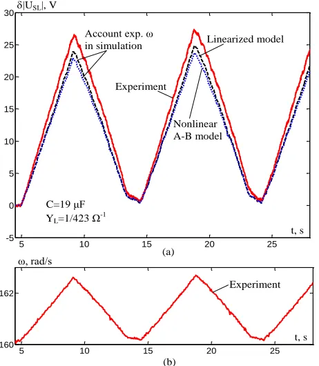
A. Validation for a Time-Varying Angular Velocity Profile The effect of a time-varying angular velocity is shown in Fig. 9 (a). The angular velocity profile is shown in Fig. 9 (b). The angular velocity was equal to 160.14 rad/s up to the start at t=5s. The voltage curves obtained from linear and nonlinear simulations are in good agreement with the experimental data.
5 10 15 20 25
160 162
5 10 15 20 25
-5 0 5 10 15 20 25 30
t, s
|USL|, V
Nonlinear A-B model
C=19 μF
YL=1/423 Ω-1
Linearized model
Experiment Account exp. ω in simulation
t, s ω, rad/s
Experiment (a)
(b)
Fig. 9. Voltage deviations caused by time varying angular velocity perturbations: (a) Simulated and experimental voltage deviations. (b) Measured angular velocity perturbations.
B. Case of Resistive-Inductive Loads
The linearized model of the SEIG with series resistive-inductive loads is derived similar to the pure resistive case following the approach in Section II.D. The derivation is based on the SEIG steady-state and dynamic analysis presented by the authors in [23]. The order of the model is 8 in this case with a state-space vector extended by two F and G load currents. The load inductance LL appears in the analysis as an
additional parameter. Fig. 10 shows the results of simulations, with voltage perturbations due to a step change of capacitance for the case of a resistive-inductive load. The curves for linearized and nonlinear models are in excellent agreement. Similar results were obtained for small perturbations ,
L
Y
, and LL.
4.9 5 5.1 5.2 5.3 5.4 5.5 5.6 5.7 5.8
-1 0 1 2 3 4 5 6 7 8
C=21 μF
YL =1/423 Ω
-1
ω=160.14 rad/s Nonlinear A-B model
t, s δC= 0.2 μF
|USL|, V
Linearized model
Step response simulation
LL =0.6524 H
Fig. 10. Voltage perturbations caused by C= 0.2 µF in the case of resistive-inductive loads.
The reduced-order state-space representation of the linearized model is similarly transformed to the corresponding transfer functions. The degrees of the polynomials in the transfer function for the capacitance disturbance input are increased by 2, so that
( ) ( )
( )
SL
C
U s
P s
C s
(21)
2 2
1 2 3 4 4
2 2 2 2 2 2
1 2 2 2 3 3 3 4 4 4
(1 )(1 )(1 )(1 2 )
(1 )(1 2 )(1 2 )(1 2 )
C C C C C C C
k T s T s T s T s T s
T s T s T s T s T s T s T s
where the parameters corresponding to the conditions of Fig. 10 are: kC 39.263V/F, TC16.1ms, TC21.6 ms,
30.831ms
C
T , TC41.5ms, C 0.887, T1124.4 ms,
21.6 ms
T , 2 0.3182, T31.4 ms, 30.896,
40.808ms
T , 4 0.123.
Note that the parameters of the transfer function Pc(s)
change significantly with the operating condition. For example, for the conditions of Fig. 6, kC 19.249V/
F andT1 = 54.4 ms (the other time constants remain significantly
[image:9.612.322.557.243.447.2] [image:9.612.60.291.447.712.2]can then be used for adaptation in the control law.
The transfer function PLL( )s USL ( ) /s L sL( ) has the
same form as P sC( ), but with different gain, time constants
and damping factors in the numerator. P s( ) has in the
numerator an additional polynomial 2 2
3 3 3
1 2 T s T s
compared to the pure resistive case. PYL( )s has a polynomial
2 2
2 2 2
1 2 YLTYL s T YL s instead of 1TYL2s for the resistive load. Note that the parameters of the transfer functions for resistive and resistive-inductive loads are labelled similarly, although their values are different.
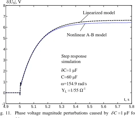
C. Applications to Larger Machines
Although the experiments of this paper were performed with a small induction machine, the theoretical results and the linear approximation are applicable to larger machines as well. To support this statement, computations and simulations were performed for a three-phase generator model from [24]. The rated values of the machine were 415V, 7.8A, 3.6 kW, and 50 Hz. The parameters of the model, adapted from [24], are given in the appendix.
4.9 5 5.1 5.2 5.3 5.4 5.5 5.6 5.7 5.8
-1 0 1 2 3 4 5 6 7 8
C=60 μF
YL =1/55 Ω-1
ω=154.9 rad/s
Nonlinear A-B model
t, s δC=1 μF
|US|, V
Linearized model
Step response simulation
Fig. 11. Phase voltage magnitude perturbations caused by C=1 µF for a larger machine.
Fig. 11 shows the transients caused by a step change of capacitance C=1 µF. The results of the linear and nonlinear models are close, validating again the linearized model. Similar results were obtained for a small decrease in capacitance, and for small angular velocity and load admittance perturbations.
The transfer functions remain the same as for the smaller machine, but with different parameter. For the conditions of Fig. 11: kC 6.648V/F, TC17.8ms, TC21.5ms,
31ms
C
T , T1122.7 ms, T21.6 ms, 20.417,
30.848ms
T , 3 0.195, kYL 10.5 10 3V/1,
113.6 ms
YL
T , TYL25.7 ms, TYL31.1ms, YL0.241,
6.118 / /
k V rad s , T138.3ms, T21.1ms,
0.275
. For possible comparison with [24], the constant
C
k is given here for a phase voltage instead of line-to-line.
V. CONCLUSIONS
The paper develops a control-oriented linearized SEIG model based on a full nonlinear model accounting for cross-saturation effect. Due to complexity and strong nonlinearity of the self-excitation phenomenon, the linearization problem does not fit the traditional theoretical framework. The objective is reached through a specific orientation of the coordinate frame that aligns it with the stator voltage vector even during transients. The model is validated through a dynamic simulation comparing to the linearized and full models, together with experimental data. The model is presented in a compact state-space form and as transfer functions suitable for systematic control system design.
APPENDIX:ANALYTIC APPROXIMATION OF MAGNETIZING
INDUCTANCE CURVE
To facilitate numerical computations, an analytic
approximation of the magnetizing curve obtained
experimentally was used. Four regions were defined, with breakpoints iM1, iM2,and iM3:
for iM<iM1 (the ascending part of the LM curve):
2 1( 1)
M MAX M M
L L b i i , (22)
where LMAX is a maximum (unsaturated) value of LM. If
LM(0)=LM0, b1(LMAXLM0) /iM21. for iM1<iM<iM2 (the flat part): LM=LMAX,
for iM2<iM<iM3(the descending part of LM curve):
3 2 1
1 2 3 4 5
M M M M M
L p i p i p i p p i , (23)
for iM>iM3:
( 3)/
3 /
iM iM iD
M MMAX MMAX M M
L e i
,
(24)where 4 3 2
3 1 3 2 3 3 3 4 3 5
M p iM p iM p iM p iM p .
From experimental data, the parameters were determined to be: LMAX=1.87 H, LM0=1 H, iM1=0.333 A, iM2=0.401 A,
b1=7.8457 H/A2, iM3=1.738 A, ΨMMAX=2.05 Wb,
p1=-0.2116 H/A3, p2=1.33 H/A2, p3=-3.203 H/A, p4=3.807 H,
p5=-0.342 HA, iD=1.414 A.
The parameters of the machine adapted from [24] are: RS=1.7Ω, RR=2.7Ω, LσS=LσR=0.0114H, np=2, LMAX=0.295 H,
LM0=0.23 H, iM1=1.2629 A, iM2=1.2657 A, b1=0.0408 H/A2,
iM3=7.0711 A, ΨMMAX=2.05 Wb,
p1=-0.00008362 H/A3, p2=0.003452 H/A2, p3=-0.05289 H/A,
p4=0.3975 H, p5=-0.05177 HA, iD=18.835 A.
ACKNOWLEDGMENT
[image:10.612.314.565.288.523.2] [image:10.612.54.291.325.531.2]REFERENCES
[1] Y.K. Chauhan, S.K. Jain, B. Singh, “A prospective on voltage regulation of self-excited induction generators for industry applications,” IEEE Trans. Industry Applications, vol. 46, no. 2, pp. 720-730, 2010.
[2] T. Chandra Sekhar, B.P. Muni, “Voltage regulators for self excited induction generator,” in Proc. IEEE Region 10 Conference TENCON, 2004, vol. C, pp. 460-463.
[3] G. Dastagir, L.A.C. Lopes, “Voltage and frequency regulation of a stand-alone self-excited induction generator,” in Proc. IEEE Canada Electrical Power Conference, 2007, pp. 502-506.
[4] K. Roy, D. Chatterjee, A.K. Ganguli, “An improved control strategy of self excited induction generator taking magnetization nonlinearity,” in Proc. International Conference on Energy, Automation, and Signal, 2011, pp. 1-5.
[5] S.N. Mahato, S.P. Singh, M.P. Sharma, “Direct vector control of stand-alone self-excited induction generator,” in Proc. Joint International Conference on Power Electronics, Drives and Energy Systems & Power India, 2010, pp. 1-6.
[6] B. Singh, S.S. Murthy, S. Gupta, “STATCOM-based voltage regulator for self-excited induction generator feeding nonlinear loads,” IEEE Trans. Ind. Electron, vol. 53, no. 5, pp. 1437–1452, 2006.
[7] R. Bonert, S. Rajakaruna, “Self-excited induction generator with excellent voltage and frequency control,” IEE Proc. Generation, Transmission and Distribution, vol. 145, issue 1, pp. 33-39, 1998. [8] G.V. Jayaramaiah, B.G. Fernandas, “Analysis of voltage regulator for a
3-Ф self-excited induction generator using current controlled voltage source inverter,” in Proc. 4th International Power Electronics and Motion Control Conference, 2004, vol. 3, pp. 1404-1408.
[9] W.-L. Chen, Y.-Hs. Lin, H.-S. Gau, and C.-H. Yu, “STATCOM controls for a self-excited induction generator feeding random loads,” IEEE Trans. Power Delivery, vol. 23, issue 4, pp. 2207-2215, 2008. [10] B. Singh, L.B. Shilpakar, “Analysis of a novel solid state voltage
regulator for a self-excited induction generator,” Proc. Inst. Elect. Eng.—Gener. Transm. Distrib., vol. 45, no. 6, pp. 647–655, 1998. [11] E. Suarez, G. Bortolotto, “Voltage-frequency control of a self-excited
induction generator,” IEEE Trans. Energy Conversion, vol. 14 , issue 3, pp. 394-401, 1999.
[12] D.T. Sepsi, R.K. Jardan, “Vector based hysteresis control for self-excited induction generators,” in Proc. 15th International Power Electronics and Motion Control Conference (EPE/PEMC), 2012, pp. DS2d.9-1 - DS2d.9-8.
[13] Hua Geng, D. Xu, Bin Wu, Wei Huang, “Direct voltage control for a stand-alone wind-driven self-excited induction generator with improved power quality,” IEEE Trans. Power Electronics, vol. 26 , issue 8, pp. 2358-2368, 2011.
[14] L. Louze, A.L. Memmour, A. Khezzar, M. Boucherma, “Input-output linearizing and sliding mode control schemes for a self-excited induction generator,” in Proc. 35th Annual Conference of IEEE Industrial Electronics, 2009, pp. 3892-3897.
[15] L. Wang, C.-H. Lee, “A novel analysis on the performance of an isolated self-excited induction generator,” IEEE Trans. Energy Conversion, vol. 12 , issue 2, pp. 109 – 117, 1997.
[16] M. Bodson, O. Kiselychnyk, J. Wang “Comparison of two magnetic saturation models of induction machines,” in Proc. IEEE International Electric Machines & Drives Conference, Chicago, IL, 2013, pp. 1004-1009.
[17] S.C. Kuo, L. Wang, “Dynamic eigenvalue analysis of a self-excited induction generator feeding an induction motor,” in Proc. IEEE Power Engineering Society Winter Meeting, 2001, vol.3, pp. 1393-1397. [18] M. Bodson, O. Kiselychnyk, “Analysis of triggered self-excitation in
induction generators and experimental validation,” IEEE Trans. Energy Conversion, vol. 27, issue 2, pp. 238–249, 2012.
[19] O. Kiselychnyk, M. Bodson, J.Wang, “Model of a self-excited induction generator for the design of capacitor-controlled voltage regulators,” in Proc. 21-st IEEE Mediterranean Conference on Control and Automation, Crete, Greece, 2013, pp. 149-154.
[20] E. Levi, “A unified approach to main flux saturation modeling in d-q axis models of induction machines,” IEEE Trans. Energy Conversion, vol. 10, no. 3, 1995, pp. 455-461.
[21] O. Kiselychnyk, M. Pushkar, M. Bodson, “Critical load of self-excited induction generators,” Electrotechnic and Computer Systems, no. 03 (79), pp. 282-285, 2011.
[22] M. Bodson, O. Kiselychnyk, “The complex Hurwitz test for the analysis of spontaneous self-excitation in induction generators,” IEEE Trans. Automatic Control, vol. 58, issue 2, pp. 449–454, 2013.
[23] O. Kiselychnyk, J. Wang, M. Bodson, M. Pushkar, “Steady-state and dynamic characteristics of self-excited induction generators with resistive-inductive loads,” in Proc. of 22 International Symposium on Power Electronics, Electrical Drives, Automation and Motion, SPEEDAM 2014, Ischia, Italy, 2014, pp. 625-630.
[24] D. Seyoum, C. Grantham, F. Rahman, “The dynamic characteristics of an isolated self-excited induction generator driven by a wind turbine,” IEEE Trans. Industry Applications, vol. 39, no. 4, 2003, pp. 936-944.
Oleh Kiselychnyk received the M.Sc. and Ph.D. degrees in Electrical Engineering and Automation from the National Technical University of Ukraine “Kiev Polytechnic Institute” (NTUU “KPI”) in 1993 and 1997 respectively. Currently, he is a Science City Research Fellow in the School of Engineering of the University of Warwick, Coventry, UK. Previously, he was a Docent of the department of electric drives of NTUU “KPI”. He was also a Visiting Fulbright Scholar at the University of Utah, USA, in 2009 and a Visiting DAAD Researcher at the Hamburg University of Technology, Germany, 2008. His main research interests are control of electric motors and generators, automation of water supply systems, and microcontrollers.
Marc Bodson received a Ph.D. degree in Electrical Engineering and Computer Science from the University of California, Berkeley, in 1986. He obtained two M.S. degrees - one in Electrical Engineering and Computer Science and the other in Aeronautics and Astronautics - from the Massachusetts Institute of Technology, Cambridge MA, in 1982. Currently, Marc Bodson is a Professor of Electrical & Computer Engineering at the University of Utah in Salt Lake City. He was Chair of the Department of Electrical & Computer Engineering between July 2003 and October 2009, and he was the Editor-in-Chief of IEEE Trans. on Control Systems Technology between January 2000 and December 2003. He was elected Fellow of the Institute of Electrical and Electronics Engineers in 2006. His research interests are in adaptive control, with applications to electromechanical systems and aerospace.