Stochastic bounds in fork join queueing systems under full and partial mapping

warwick.ac.uk/lib-publications

Original citation:

Rizk, Amr, Poloczek , Felix and Ciucu, Florin. (2016) Stochastic bounds in fork-join queueing

systems under full and partial mapping. Queueing Systems, 83 (3). pp. 261-291.

Permanent WRAP URL:

http://wrap.warwick.ac.uk/79510

Copyright and reuse:

The Warwick Research Archive Portal (WRAP) makes this work by researchers of the

University of Warwick available open access under the following conditions. Copyright ©

and all moral rights to the version of the paper presented here belong to the individual

author(s) and/or other copyright owners. To the extent reasonable and practicable the

material made available in WRAP has been checked for eligibility before being made

available.

Copies of full items can be used for personal research or study, educational, or not-for profit

purposes without prior permission or charge. Provided that the authors, title and full

bibliographic details are credited, a hyperlink and/or URL is given for the original metadata

page and the content is not changed in any way.

Publisher’s statement:

“The final publication is available at Springer via

http://dx.doi.org/10.1007/s11134-016-9486-x

A note on versions:

The version presented here may differ from the published version or, version of record, if

you wish to cite this item you are advised to consult the publisher’s version. Please see the

‘permanent WRAP URL’ above for details on accessing the published version and note that

access may require a subscription.

(will be inserted by the editor)

Stochastic Bounds in Fork-Join Queueing Systems

under Full and Partial Mapping

Amr Rizk · Felix Poloczek · Florin Ciucu

the date of receipt and acceptance should be inserted later

Abstract In a Fork-Join (FJ) queueing system an upstream fork station splits incoming jobs intoN tasks to be further processed byN parallel servers, each with its own queue; the response time of one job is determined, at a down-stream join station, by the maximum of the corresponding tasks’ response times. This queueing system is useful to the modelling of multi-service sys-tems subject to synchronization constraints, such as MapReduce clusters or multipath routing. Despite their apparent simplicity, FJ systems are hard to analyze.

This paper provides the firstcomputable stochastic bounds on the waiting and response time distributions in FJ systems under full (bijective) and partial (injective) mapping of tasks to servers. We consider four practical scenarios by combining 1a) renewal and 1b) non-renewal arrivals, and 2a) non-blocking and 2b) blocking servers. In the case of non-blocking servers we prove that delays scale as O(logN), a law which is known for first moments under renewal input only. In the case of blocking servers, we prove that the same factor of logN dictates the stability region of the system. Simulation results indicate that our bounds are tight, especially at high utilizations, in all four scenarios. A remarkable insight gained from our results is that, at moderate to high utilizations, multipath routing “makes sense” from a queueing perspective for two paths only, i.e., response times drop the most whenN = 2; the technical

Amr Rizk

University of Massachusetts Amherst, USA E-mail: [email protected]

Felix Poloczek

University of Warwick, UK / TU Berlin, Germany E-mail: [email protected]

Florin Ciucu

explanation is that the resequencing (delay) price starts to quickly dominate the tempting gain due to multipath transmissions.

Keywords Fork-Join queue · Performance evaluation · Parallel systems ·

MapReduce·Multipath

1 Introduction

The performance analysis of Fork-Join (FJ) systems received new momentum with the recent wide-scale deployment of large-scale data processing that was enabled through emerging frameworks such as MapReduce [13]. The main idea behind these big data analysis frameworks is an elegant divide and conquer strategy with various degrees of freedom in the implementation. The open-source implementation of MapReduce, known as Hadoop [42], is deployed in numerous production clusters, e.g., Facebook and Yahoo [24].

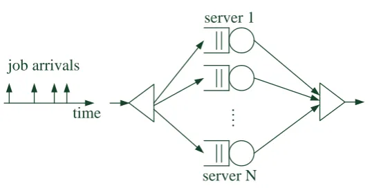
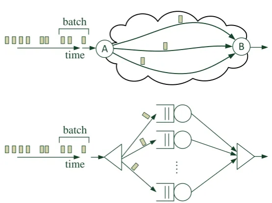
The basic operation of MapReduce is depicted in Figure 1. In the map phase, a job is split into multiple tasks that are mapped to different workers (servers). Once a specific subset of these tasks finish their executions, the corresponding reduce phase starts by processing the combined output from all the corresponding tasks. In other words, the reduce phase is subject to a fundamental synchronization constraint on the finishing times of all involved tasks.

A natural way to model one reduce phase operation is by abasicFJ queue-ing system with N servers. Jobs, i.e., the input unit of work in MapReduce systems, arrive according to some point process. Each job is split intoN(map) tasks (orsplits, in the MapReduce terminology), which are simultaneously sent to the N servers. At each server, each task requires a random service time, capturing the variable task execution times on different servers in the map phase. A job leaves the FJ system when all of its tasks are served; this con-straint corresponds to the specification that the reduce phase starts no sooner than when all of its map tasks complete their executions.

Concerning the execution of tasks belonging to different jobs on the same server, there are two operational modes. In thenon-blockingmode, the servers are workconserving in the sense that tasks immediately start their executions once the previous tasks finish theirs. In theblocking mode, the mapped tasks of a job simultaneously start their executions, i.e., servers can be idle when their corresponding queues are not empty. The non-blocking execution mode prevails in MapReduce due to its conceivable efficiency, whereas the blocking execution mode is employed when the jobtracker (the node coordinating and scheduling jobs) waits for all machines to be ready to synchronize the configuration files before mapping a new job; in Hadoop, this can be enforced through the coordination servicezookeeper[42].

first non-asymptotic and computable stochastic bounds on the waiting and response time distributions in the most relevant scenario, i.e., non-renewal (Markov modulated) job arrivals and the non-blocking operational mode. Un-der all scenarios, the bounds are numerically tight especially at high utiliza-tions. This inherent tightness is due to a suitable martingale representation of the underlying queueing system, an approach which was conceived in [27] for the analysis of GI/GI/1 queues, and which was recently extended to address multi-class queues with non-renewal arrivals [12, 34]. The simplicity of the ob-tained stochastic bounds enables the derivation of scaling laws, e.g., delays in FJ systems scale as O(logN) in the number of parallel servers N, for both renewal and non-renewal arrivals, in the non-blocking mode; more severe delay degradations hold in the blocking mode, and, moreover, the stability region depends on the same fundamental factor of logN.

In addition to the direct applicability to the dimensioning of MapReduce clusters, there are other relevant types of parallel and distributed systems such as production or supply networks. In particular, by slightly modifying the basic FJ system corresponding to MapReduce, the resulting model suits the analysis of window-based transmission protocols over multipath routing. By making several simplifying assumptions such as ignoring the details of specific protocols (e.g., multipath TCP), we can provide a fundamental understanding of multipath routing from a queueing perspective. Concretely, we demonstrate that sending a flow of packets over two paths, instead of one, does generally reduce the steady-state response times. The surprising result is that by sending the flow over more than two paths, the steady-state response times start to increase. The technical explanation for such a rather counterintuitive result is that the logN resequencing price at the destination quickly dominates the tempting gain in the queueing waiting time due to multipath transmissions.

The rest of the paper is structured as follows. We first discuss related work on FJ systems and related applications. Then we analyze full mapping, i.e., a mapping of jobs to N servers in Sections 3 and 4. We analyze both non-blocking and blocking FJ systems with renewal input in Section 3, and with non-renewal input in Section 4. The analysis of partial mapping, i.e., a mapping of jobs toH≤N servers follows in Section 5. In Section 6 we apply the obtained results on the steady-state response time distributions to the analysis of multipath routing from a queueing perspective. Brief conclusions are presented in Section 7.

2 Related Work

We first review analytical results on FJ systems, and then results related to the two application case studies considered in this paper, i.e., MapReduce and multipath routing.

map

map

map

map

reduce

reduce input job

split 1

split n

Fig. 1 Schematic illustration of the basic operation of MapReduce.

[5, 31, 40, 25, 28, 6, 8]. In particular, [5] notes that an exact performance eval-uation of general FJ systems is remarkably hard due to the synchronization constraints on the input and output streams. More precisely, a major difficulty lies in finding an exact closed form expression for the joint steady-state work-load distribution for the FJ queueing system. However, a number of results exist given certain constraints on the FJ system. The authors of [15] provide the stationary joint workload distribution for a two-server FJ system under Poisson arrivals and independent exponential service times. For the general case of more than two parallel servers there exists a number of works that pro-vide approximations [31, 40, 28, 29] and bounds [5, 6] for certain performance metrics of the FJ system. Given renewal arrivals, [6] significantly improves the lower bounds from [5] in the case of heterogeneous phase-type servers using a matrix-geometric algorithmic method. The authors of [28] provide an ap-proximation of the sojourn time distribution in a renewal driven FJ system consisting of multiple G/M/1 nodes. They show that the approximation er-ror diminishes at extremal utilizations. Refined approximations for the mean sojourn time in two-server FJ systems that take the first two moments of the service time distribution are given in [25]; numerical evidence is further provided on the quality of the approximation for different service time distri-butions. In a recent work, the authors of [30] establish Gaussian limits for the joint distributions of the service and waiting times for synchronization under general arrivals characterized by a limiting Brownian motion.

also holds in the case of Markov modulated arrivals. In a parallel work [26] to ours, the authors adopt a network calculus approach to derive stochastic bounds in a non-blocking FJ system, under a strong assumption on the input; for related constructions of such arrival models see [20].

The work in [21, 22] studies FJ systems where jobs leave the system when a subset H ≤N of its tasks are finished. This system is similar to the par-tial mapping FJ system that we study in Section 5, however, with subtle yet fundamental differences. The FJ system presented in [21, 22] is based on the assumption that when H tasks finish execution, the finished job purges the unfinishedN −H tasks out their corresponding queues. The authors of [21, 22] provide upper bounds for the mean response times in such systems under Poisson arrivals and general service distributions. In Section 5, we consider in-stead injective task mapping, i.e., jobs areonlyforked onto a subset of servers

H ≤N. For this type of FJ systems we provide bounds on the steady state waiting and response time distributions under round-robin and random task placement.

Concerning concrete applications of FJ systems, in particular MapReduce, there are several empirical and analytical studies analyzing its performance. For instance, [44, 3] aim to improve the system performance via empirically adjusting its numerous and highly complex parameters. The targeted perfor-mance metric in these studies is the job response time, which is in fact an integral part of the business model of MapReduce based query systems such as [32] and time priced computing clouds such as Amazon’s EC2 [1]. For an overview on works that optimize the performance of MapReduce systems see the survey article [33]. Using a similar idea as in [5], the authors of [37] derive asymptotic results on the response time distribution in the case of renewal arrivals; such results are further used to understand the impact of different scheduling models in the reduce phase of MapReduce. Using the model from [37] the work in [38] provides approximations for the number of jobs in a tan-dem system consisting of a map queue and a reduce queue in the heavy traffic regime. The work in [41] derives approximations of the mean response time in MapReduce systems using a mean value analysis technique and a closed FJ queueing system model from [39].

multipath routing, motivated by the emerging application of multipath TCP [35]. We point out, however, that we do not model the specific operation of any particular multipath transmission protocol. Instead, we analyze a generic multipath transmission protocol under simplifying assumptions, in order to provide a theoretical understanding of the overall response times comprised of both queueing and resequencing delays.

Relative to the existing literature, our key theoretical contribution is to provide computable and non-asymptotic bounds on the distributions of the steady-state waiting and response times under bothrenewal andnon-renewal

input in non-blocking FJ systems. These bounds can be found in Theorem 1, Theorem 3, and Theorem 5 – Theorem 7. The consideration of non-renewal input is particularly relevant, given recent observations that job arrivals are subject to temporal correlations in production clusters. For instance, [11, 23] report that job, respectively, flow arrival traces in clusters running MapRe-duce exhibit various degrees of burstiness. We augment the scope of the main contributions in this work by consideringblocking FJ systems that essentially correspond to GI/G/1 queueing systems. Here, we recover and extend promi-nent results, e.g., from [2, 16] in Theorem 2 and Theorem 4, respectively. Note that non-blocking FJ systems behave fundamentally different from blocking FJ systems, thus requiring adapted mathematical tools for the analysis.

3 FJ Systems with Renewal Input

We consider a FJ queueing system as depicted in Figure 2. Jobs arrive at the input queue of the FJ system according to some point process with interarrival times ti between the i and i+ 1 jobs. Each job i is split into N tasks that

are mapped through a bijection toN servers. A task of jobithat is serviced by some server n requires a random service timexn,i. A job leaves the

sys-tem when all of its tasks finish their executions, i.e., there is an underlying synchronization constraint on the output of the system. We assume that the families{ti} and{xn,i}are independent.

In the sequel we differentiate between two cases, i.e., a) non-blocking and

b) blocking servers. The first case corresponds to workconserving servers, i.e., a server starts servicing a task of the next job (if available) immediately upon finishing the current task. In the latter case, a server that finishes servicing a task is blocked until the corresponding job leaves the system, i.e., until the last task of the current job completes its execution. This can be regarded as an additional synchronization constraint on the input of the system, i.e., all tasks of a job start receiving service simultaneously. We will next analyzea) andb) for renewal arrivals.

3.1 Non-Blocking Systems

Consider an arrival flow of jobs with renewal interarrival timesti, and assume

job arrivals

…

.

time

server 1

server N

Fig. 2 A schematic Fork-Join queueing system withN parallel servers. An arriving job is split intoN tasks, one for each server. A job leaves the FJ system when all of its tasks are served. An arriving job is considered waiting until the service of the last of its tasks starts, i.e., when the previous job departs the system.

waiting time wj of thejth job is defined as

wj = max (

0, max 1≤k≤j−1

(

max

n∈[1,N]

( k X

i=1

xn,j−i− k X

i=1 tj−i

)))

, (1)

for all j ≥ 2, where xn,j is the service time required by the task of job j

that is mapped to server n. We count a job as waiting until its last task starts receiving service. Similarly, the response times of jobs, i.e., the times until the last corresponding tasks have finished their executions, are defined asr1= maxnxn,1for the first job, and forj≥2 as

rj = max

0≤k≤j−1

(

max

n∈[1,N]

( k X

i=0

xn,j−i− k X

i=1 tj−i

))

, (2)

where by conventionP0

i=1ti = 0; for brevity, we will denote maxn:= maxn∈[1,N]. We assume that the task service timesxn,jare independent and identically

distributed (iid). The stability condition for the FJ queueing system is given as E[x1,1]< E[t1]. By stationarity and reversibility of the iid processes xn,j

and tj, there exists a distribution of the steady-state waiting time w and

steady-state response timer, respectively, which have the representations

w=Dmax

k≥0 ( max n ( k X i=1 xn,i−

k X i=1 ti )) (3) and

r=Dmax

k≥0 ( max n ( k X i=0 xn,i−

k X i=1 ti )) , (4)

The following theorem provides stochastic upper bounds onwandr. The corresponding proof will rely on submartingale constructions and the Optional Sampling Theorem (see Lemma 1 in the Appendix).

Theorem 1 _{(Renewals, Non-Blocking)}Given a FJ system withN paral-lel non-blocking servers that is fed by renewal job arrivals with interarrivalstj.

If the task service timesxn,jare iid, then the steady-state waiting and response

timesw andrare bounded by

P[w≥σ]≤N e−θnbσ ₍₅₎

P[r≥σ]≤NE

eθnbx1,1

e−θnbσ _{, (6)}

where θnb (with the subscript ‘nb’ standing for non-blocking) is the (positive)

solution of

E

eθx1,1_Ee−θt1_{= 1 . (7)}

We remark that the stability condition E[x1,1] < E[t1] guarantees the existence of a positive solution in (7) (see also [34]).

Proof Consider the waiting timew. We first prove that for eachn∈[1, N] the process

zn(k) =eθnb

Pk

i=1(xn,i−ti)

is a martingale with respect to the filtration

Fk:=σ{xn,m, tm|m≤k, n∈[1, N]} .

The independence assumption ofxn,j andtj implies that

E[zn(k)| Fk−1] =E

h

eθnbPki=1(xn,i−ti) Fk−1

i

=Eheθnb(xn,k−tk)i_eθnbPki=1−1(xn,i−ti)

=eθnbPik=1−1(xn,i−ti)

=zn(k−1), (8)

under the condition on θnb from the theorem. Moreover, zn(k) is obviously

integrable by the condition on θnb from the theorem, completing thus the

proof for the martingale property. Next we prove that the process

z(k) = max

n zn(k) (9)

is a submartingale w.r.t.Fk. Given the martingale property of each of thezn

and the monotonicity of the conditional expectation we can write forj∈[1, N]:

Ehmax

n zn(k) Fk−1

i

where the inequality stems from maxnzn(k)≥zj(k) forj∈[1, N] a.s., whereas

the subsequent equality stems from the martingale property (8) forzn(k) for

alln∈[1, N]. Hence, we can write

E[z(k)| Fk−1]≥max

n zn(k−1) =z(k−1), (10)

which proves the submartingale property.

To derive a bound on the steady-state waiting time distribution, let σ >0 and define the stopping time

K:= inf

(

k≥0

max

n k X

i=1

(xn,i−ti)≥σ )

, (11)

which is also the first point in timek wherez(k)≥eθnbσ_{. Note that with the}

representation ofwfrom (3):

{K <∞}={w≥σ}.

Now, using the Optional Sampling Theorem (see Lemma 1 from the Appendix) for submartingales withk≥1:

N = X

n∈[1,N]

EheθnbPki=1(xn,i−ti) i

≥Ehmax

n e

θnbPki=1(xn,i−ti) i

(12)

=E[z(k)]≥E[z(K∧k)]≥E[z(K)1K<k] ≥eθnbσ_{P[K < k] ,}

where we used the condition onθnbfrom the theorem in the first line, the union

bound in the second line, and the submartingale property in the third line. In the last line we used the definition of the stopping timeK; note that we use the notationK∧n:= min{K, n}. The proof completes by lettingk→ ∞.

For the response timer, define the processes

˜

zn(k) =eθnb(

Pk

i=0xn,i−Pki=1ti)_,

which differs from the zn only in the range of the sum of the service times xn,i. Then we proceed as for the derivation of the bound on the waiting time w. The only difference in the derivation is that inequality (12) translates to

NE

eθnbx1,1

≥Ehmax

n e

θnb(Pki=0xn,i−Pki=1ti)i _.

the impact of a MapReduce server pool size N on the job waiting/response times.

We note that the bound in Theorem 1 can be computed for different ar-rival and service time distributions as long as the MGF (moment generating function) and Laplace transform from (7) are computable. Given a scenario where the job interarrival process and the task size distributions in a MapRe-duce cluster are not known a priori, estimates of the corresponding MGF and Laplace transforms can be obtained using recorded traces, e.g., using the method from [17].

Next we illustrate two immediate applications of Theorem 1.

Example 1: Exponentially distributed interarrival and service times

Consider that the interarrival timestiand service timesxn,i are exponentially

distributed with parameters λ and µ, respectively; note that when N = 1 the system corresponds to the M/M/1 queue. The corresponding stability condition becomesµ > λ. Using Theorem 1, the bounds on the steady-state waiting and response time distributions are

P[w≥σ]≤N e−(µ−λ)σ (13)

and

P[r≥σ]≤ N ρe

−(µ−λ)σ _{, (14)}

where the exponential decay rate µ−λ follows by solving _µ−µ_θλ+λ_θ = 1, i.e., the instantiation of (7). Here, we useρto denote the utilizationλ/µ.

Next we briefly compare our results to the existing bound on the mean response time from [5], given as

E[r]≤ 1 µ−λ

N X

n=1 1

n . (15)

By integrating the tail of (14) we obtain the following upper bound on the mean response time

E[r]≤ log(N/ρ) + 1

µ−λ .

Compared to (15), our bound exhibits the same logNscaling law but is numer-ically slightly looser; asymptotnumer-ically inN, the ratio between the two bounds converges to one. A key technical reason for obtaining a looser bound is that we mainly focus on deriving bounds on distributions; through integration, the numerical discrepancies accumulate.

waiting time

probability

ρ =0.9

ρ =0.75

ρ =0.5

0 25 50 75 100 125 150

10

−6

10

−4

10

−2

10

0

(a) Non-Blocking

waiting time

probability

ρ =0.9

ρ =0.75

ρ =0.5

0 25 50 75 100 125 150

10

−6

10

−4

10

−2

10

0

(b) Blocking

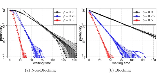
Fig. 3 Bounds on the waiting time distributions vs. simulations (renewal input): (a) the non-blocking case (13) and (b) the blocking case (22). The system parameters areN= 20,

µ= 1, and three utilization levelsρ={0.9,0.75,0.5} (from top to bottom). Simulations include 100 runs, each accounting for 107 slots.

Example 2: Exponentially distributed interarrival times and constant service times

We now consider the case of iid exponentially distributed interarrival timesti

with parameter λ, and deterministic service times xn,i = 1/µ, for all i ≥ 0

andn∈[1, N]; note that whenN = 1 the system corresponds to the M/D/1 queue.

The condition on the asymptotic decay rateθnb from Theorem 1 becomes

λ λ+θnb

=e−θnbµ _,

which can be numerically solved; upper bounds on the waiting and response time distributions follow then immediately from Theorem 1.

3.2 Blocking Systems

Here, we consider a blocking FJ queueing system, i.e., the start of each job is synchronized amongst all servers. We maintain the iid assumptions on the interarrival times ti and service times xn,i. The waiting time and response

time for thejth job can then be written as

wj = max (

0, max 1≤k≤j−1

( k X

i=1 max

n xn,j−i− k X

i=1 tj−i

))

rj = max

0≤k≤j−1

( k X

i=0 max

n xn,j−i− k X

i=1 tj−i

)

Note that the only difference to (1) and (2) is that the maximum over the number of servers now occurs inside the sum. Note that this blocking system corresponds to a GI/GI/1 queue which is analyzed, e.g., in [2].

It is evident that the blocking system is more conservative than the blocking system in the sense that the waiting time distribution of the non-blocking system is dominated by the waiting time distribution of the non-blocking system. Moreover, the stability region for the blocking system, given byE[t1]>

E[maxnxn,1], is included in the stability region of the corresponding non-blocking system (i.e.,E[t1]>E[x1,1]).

Analogously to (3), the steady-state waiting and response times w and r

have now the representations

w=Dmax

k≥0

( k X

i=1 max

n xn,i− k X

i=1 ti

)

(16)

r=Dmax

k≥0

( k X

i=0 max

n xn,i− k X

i=1 ti

)

. (17)

The following theorem provides upper bounds onwandr.

Theorem 2 _{(Renewals, Blocking)} Given a FJ queueing system with N

parallel blocking servers that is fed by renewal job arrivals with interarrivals

tj and iid task service timesxn,j. The distributions of the steady-state waiting

and response times are bounded by

P[w≥σ]≤e−θbσ ₍₁₈₎

P[r≥σ]≤E

eθbmaxnx1,1 e−θbσ _,

whereθb(with the subscript ‘b’ standing for blocking) is the (positive) solution

of

E

eθmaxnxn,1_Ee−θt1_{= 1 . (19)}

Before giving the proof we note that, in general, (19) can be numerically solved. Moreover, for small values ofN,θb can be analytically solved.

Proof Consider the waiting time w. We proceed similarly as in the proof of Theorem 1. LettingFk as above, we first prove that the process

y(k) =eθbPik=1(maxnxn,i−ti)

is a martingale w.r.t.Fk using a technique from [27]. We write

E[y(k)| Fk−1] =E

h

eθbPki=1(maxnxn,i−ti) Fk−1

i

=eθbPki=1−1(maxnxn,i−ti)_Eh_eθb(maxnxn,k−tk)i

=eθbPik=1−1(maxnxn,i−ti)

where we used the independence and renewal assumptions forxn,i andti in

the second line, and finally the condition onθb from (19).

In the next step we apply the Optional Sampling Theorem (45) to derive the bound from the theorem. We first define the stopping timeK by

K:= inf

(

k≥0

k X

i=1

max

n xn,i−ti

≥σ )

. (20)

Recall thatP[K <∞] =P[w≥σ]. We can next write for everyk∈_N

1 =E[y(0)] =E[y(K∧k)]

≥E[y(K∧k)1K<k]

=EheθbPKi=1(maxnxn,i−ti)₁ K<k

i

≥eθbσ_{P[K < k] .}

Taking k → ∞ completes the proof. The proof for the response time r is analogous.

Example 3: Exponentially distributed interarrival and service times

Consider interarrival and service timesti andxn,i that are exponentially

dis-tributed with parametersλandµ, respectively. In [36] it was shown that

max

n Ln=D N X

n=1 Ln

n

for iid exponentially distributed random variables Ln, so that the stability

conditionE[t1]>E[maxnxn,1] becomes

1

λ >

1

µ N X

n=1 1

n . (21)

By applying Theorem 2, the bounds on the steady-state waiting and re-sponse time distributions are

P[w≥σ]≤e−θbσ ₍₂₂₎

and

P[r≥σ]≤ µ µ−θb

e−θbσ _,

whereθb can be numerically solved from the condition

N Y

n=1 nµ nµ−θb

λ λ+θb

For quick numerical illustrations we refer back to Figure 3.(b).

The interesting observation is that the stability condition from (21) de-pends on the number of serversN. In particular, as the right hand side grows in logN, the system becomes unstable (i.e., waiting times are infinite) for suf-ficiently large N. This shows that the optional blocking mode from Hadoop should be judiciously enabled.

Example 4: Exponentially distributed interarrival and constant service times

If the service times are deterministic, i.e., xn,i = 1/µ for all i ≥ 0 andn ∈

[1, N], the representations of w and r from (16) and (17) match their non-blocking counterparts from (3) and (4) and hence the corresponding stability regions and stochastic bounds are equal to those from Example 2.

4 FJ Systems with Non-renewal Input

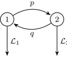
In this section we consider the more realistic case of FJ queueing systems with non-renewal job arrivals. This model is particularly relevant given the empirical evidence that clusters running MapReduce exhibit various degrees of burstiness in the input [11, 23]. Moreover, numerous studies have demonstrated the burstiness of Internet traces, which can be regarded in particular as the input to multipath routing.

1 2

p

q

L1 L2

Fig. 4 Markov modulating chainckfor the job interarrival times.

We model the interarrival times ti using a Markov modulated process.

Concretely, consider a two-state modulating Markov chainck, as depicted in

Figure 4, with a transition matrixT given by

T =

1−p p

q 1−q

, (23)

for some values 0< p, q <1. In statei∈ {1,2}the interarrival times are given by iid random variablesLi with distributionLi. Without loss of generality we

assume thatL1 is stochastically smaller thanL2, i.e.,

for anyt≥0. Additionally, we assume that the Markov chainck satisfies the

burstiness condition

p <1−q , (24)

i.e., the probability of jumping to a different state is less than the probability of staying in the same state.

Subsequent derivations will exploit the following exponential transform of the transition matrixT defined as

Tθ:=

(1−p)Ee−θL1 _{p Ee}−θL2

q Ee−θL1_(1−q)Ee−θL2

,

for some θ >0. Let Λ(θ) denote the maximal positive eigenvalue of Tθ, and

the vectorh= (h(1), h(2)) denote a corresponding eigenvector. By the Perron-Frobenius Theorem,Λ(θ) is equal to the spectral radius ofTθsuch thathcan

be chosen with strictly positive components.

As in the case of renewal arrivals, we will next analyze both non-blocking and blocking FJ systems.

4.1 Non-Blocking Systems

We first analyze a non-blocking FJ system fed with arrivals that are modulated by a stationary Markov chain as in Figure 4. We assume that the task service timesxn,j are iid and that the families{ti}and{xn,i} are independent. Note

that both the definition of wj from (1) and the representation of the

steady-state waiting timewin (3) remain valid, due to stationarity and reversibility; the same holds for the response times.

The next theorem provides upper bounds on the steady-state waiting and response time distributions in the non-blocking scenario with Markov modu-lated interarrivals.

Theorem 3 (Non-Renewals, Non-Blocking) Given a FJ queueing sys-tem withN parallel non-blocking servers, Markov modulated job interarrivals

tj according to the Markov chain depicted in Figure 4 with transition matrix

(23), and iid task service times xn,j. The steady-state waiting and response

time distributions are bounded by

P[w≥σ]≤N e−θnbσ ₍₂₅₎

P[r≥σ]≤NE

eθnbx1,1_e−θnbσ _{, (26)}

where θnbis the (positive) solution of

Eeθx1,1_{Λ(θ) = 1.}

(Recall thatΛ(θ)was defined as a spectral radius.)

We remark that the existence of a positive solution θnb is guaranteed by

Proof Consider the filtration

Fk:=σ{xn,m, tm, cm|m≤k, n∈[1, N]} ,

that includes information about the state ck of the Markov chain. Now, we

construct the processz(k) as

z(k) =h(ck)eθnb(maxn

Pk

i=1xn,i−Pki=1ti)

=eθnb(maxnPik=1xn,i−kD) _h(c

k)eθnb(kD−

Pk

i=1ti) ₍₂₇₎

with the deterministic parameter

D:=θ_nb−1log Eeθnbx1,1 _.

Note the similarity ofz(k) to (9) except for the additional functionh. Roughly, the functionhcaptures the correlation structure of the non-renewal interarrival time process.

Next we show that both terms of (27) are submartingales. In the first step we note that by the definition ofD:

Eheθnb(Pik=1xn,i−kD) Fk−1

i

=eθnb(Pik=1−1xn,i−(k−1)D) _,

hence, following the line of argument in (10) the left factor of (27), which accounts for the additional maxn, is a submartingale. The second step is similar

to the derivations in [10, 14]. First, note that

Ehh(ck)eθnb(D−tk) Fk−1

i

=eθnbD_T

θnbh(ck−1)

=eθnbD_Λ(θ

nb)h(ck−1)

=h(ck−1), (28)

where the last line is due to the definitions of D and θnb. Now, multiplying

both sides of (28) by eθnb((k−1)D−Pki=1−1ti) proves the martingale and hence

the submartingale property of the right factor in (27). As the processz(k) is a product of two independent submartingales, it is a submartingale itself w.r.t.

Fk.

Next, we derive a bound on the steady-state waiting time distribution using the Optional Stopping Theorem. Here, we use the stopping timeKdefined in (11). Recall that P[K <∞] = P[w≥σ]. On the one hand we can write for everyk∈N

E[z(k)]≥E[z(K∧k)]

≥E[z(K∧k)1K<k]

=Ehmax

n h(cK)e

θnb(PKi=1xn,i−PKi=1ti)1 K<k

i

≥eθnbσ_E[h(c

K)1K<k]

=eθnbσ_E[h(c

number of servers

percentile

ε =10−4

ε =10−3

ε =10−2

0 5 10 15 20

0

10

20

30

40

50

60

(a) Impact ofε

number of servers

percentile

p+q=0.1

p+q=0.9

0 5 10 15 20

0

10

20

30

40

50

60

(b) Impact of the burstiness factorp+q

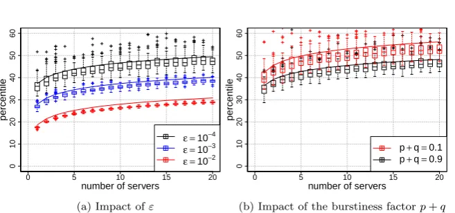
Fig. 5 TheO(logN) scaling of waiting time percentileswε _{for Markov modulated input}

(the non-blocking case (25)). The system parameters areµ= 1, λ2= 0.9, ρ= 0.75 (in both (a) and (b))p= 0.1, q= 0.4 (in (a)), three violation probabilitiesε(in (a)),ε= 10−4 _and only two burstiness parametersp+q(in (b)) (for visual convenience). Simulations include 100 runs, each accounting for 107_slots.

On the other hand we can upper bound the term

E[z(k)] =Ehmax

n e

θnb(Pki=1xn,i−kD)i_Eh_h(c

k)eθnb(kD−

Pk i=1ti)i

≤NE[h(c1)] .

Lettingk→ ∞in (29) leads to

P[K <∞]≤ E[h(c1)]

E[h(cK)|K <∞]

N e−θnbσ _{. (30)}

In Lemma 2 it is shown that the distribution of the random variable (cK | K < k) is stochastically smaller than the stationary distribution of the Markov chain. Given the burstiness condition in (24) and that the functionhis mono-tonically decreasing [9], we can further upper bound the prefactor in (30) as

E[h(c1)]

E[h(cK)|K <∞] ≤1,

which completes the proof. The proof for the response timeris analogous.

Remark: Note that, if the burstiness condition (24) is not fulfilled then we can still upper bound the prefactor in (30) using the trivial upper bound

E[h(c1)]

E[h(cK)|K <∞]

≤ E[h(c1)]

minkh(ck) .

Figure 5 displays the bounds on the waiting time percentileswε_{, for various}

4.2 Blocking Systems

Now we turn to the blocking variant of the FJ system that is fed by the same non-renewal arrivals as in the previous section. In the following, we consider exponential distributionsLmform∈ {1,2}. The main result is:

Theorem 4 _{(Non-Renewals, Blocking)}Given a FJ system withN block-ing servers, Markov modulated job interarrivals tj, and iid task service times xn,j. The steady-state waiting and response time distributions are bounded by

P[w≥σ]≤e−θbσ ₍₃₁₎

P[r≥σ]≤Eeθbmaxnx1,1_e−θbσ _,

where θb is the (positive) solution of

E

eθmaxnxn,1_{Λ(θ) = 1 .}

We remark that the positive solution forθbis guaranteed under the stronger

stability conditionE[t1]>E[maxnxn,1] and the Perron-Frobenius Theorem.

Proof LetD:=θ−1_b logEeθbmaxnxn,1_{and define the process yby:}

y(k) =h(ck)eθb(

Pk

i=1maxnxn,i−Pki=1ti)

= (eθb(Pki=1maxnxn,i−kD))(_h(c

k)eθb(kD−

Pk i=1ti))_.

Similarly to the proofs of Theorem 2 and Theorem 3 one can show that both the first and second factor ofy are martingales, and hencey is a martingale. We use the stopping timeK in (20) and write

E[h(c1)] =E[y(0)] ≥E[y(K∧k)]

≥E[y(K∧k)1K<k]

=Eheθb(PKi=1maxnxn,i−PKi=1ti)_h(c

K)1K<k i

≥eθbσ_E[h(c

K)|K <∞]P[K < k] .

Takingk→ ∞we obtain the bound

P[K <∞]≤ E[h(c1)]

E[h(cK)|K <∞]

e−θbσ_≤e−θbσ _,

where we used Lemma 2 for the last inequality. The proof forris analogous.

A close comparison of the waiting time bound in the non-renewal case (31) to the corresponding bound in the renewal case (18) reveals that the decay factorsθb depend on similar conditions, whereby the MGF of the interarrival

waiting time

probability

ρ =0.9

ρ =0.75

ρ =0.5

0 25 50 75 100 125 150

10

−6

10

−4

10

−2

10

0

(a) Non-Blocking

waiting time

probability

ρ =0.9

ρ =0.75

ρ =0.5

0 25 50 75 100 125 150

10

−6

10

−4

10

−2

10

0

(b) Blocking

Fig. 6 Bounds on the waiting time distributions vs. simulations (non-renewal input): (a) the non-blocking case (25) and (b) the blocking case (31). The parameters areN= 20, µ= 1, p = 0.1, q = 0.4, λ1 ∈ {0.4,0.72,0.72} and λ2 ∈ {0.9,0.9,1.62} leading to utilizations

ρ∈ {0.5,0.75,0.9}. Simulations include 100 runs, each accounting for 107 _slots.

the blocking system with non-renewal input is subject to the same degrading stability region (in logN) as in the renewal case (recall (21)).

For quick numerical illustrations of the tightness of the bounds on the waiting time distributions in both the non-blocking and blocking cases we refer to Figure 6.

So far we have contributed stochastic bounds on the steady-state waiting and response time distributions in FJ systems fed with either renewal and non-renewal job arrivals. The key technical insight was that the stochastic bounds in the non-blocking model grow asO(logN) in the number of parallel serversNunder non-renewal arrivals, which extends a known result for renewal arrivals [31, 5]. The same fundamental factor of logN was shown to drive the stability region in the blocking model. A concrete application follows next.

5 Partial Mapping

restrict the exposition to the more interesting case of non-blocking servers since most of the derivations rely on results from Sections 3 and 4.

5.1 Round-robin Partial Mapping, Dyadic System

We consider a dyadic FJ system where the number of servers is given as

N = 2W _{(withW ≥1) and a job is split intoH = 2}V _{tasks (with 1≤V ≤W).}

The assignment of tasks to servers follows a round-robin scheme such that the first job is assigned to servers 1, . . . , H, the second to the serversH+1, . . . ,2H, etc.

In the following, we consider job arrivals as renewal processes similar to Sect. 3. For the analysis it is sufficient to look only at an equivalent “FJ subsystem” that consists of only H servers and adjust the job interarrival times ¯tk to that system accordingly:

¯

tk :=

2(W−V)

X

i=1

t(k−1)2(W−V)_+i .

Note that for the extremal caseV =W we recover the scenario from Sect. 3, i.e., ¯tk=tk.

The Laplace transform of the job interarrival times ¯tk to one subsystem is

obtained directly from the Laplace transform of the original job interarrival timestk and the number of subsystems:

Ehe−θ¯t1i_=Ee−θt12

W−V

=Ee−θt1

N H _.

The steady-state waiting time distribution now has the following represen-tation:

w=D max

k≥0

(

max 1≤n≤H

( k X

i=1 xn,i−

k X

i=1 ¯

ti ))

(32)

and the response time:

r=Dmax

k≥0

(

max 1≤n≤H

( _k X

i=0 xn,i−

k X

i=1 ¯

ti ))

. (33)

The next theorem provides upper bounds on the steady-state waiting and response time distributions in the non-blocking scenario with partial round-robin mapping and renewal interarrivals.

Theorem 5 _{(round-robin mapping, Renewals, Non-Blocking)} Given a FJ queueing system with N = 2W _{non-blocking servers and partial}

round-robin mapping of jobs toH = 2V _{servers with1≤V ≤W. The system is fed}

by renewal job arrivals with interarrivalstj. If the input job size is normalized

service times xn,i being iid, then the steady-state waiting and response times wandr are bounded by

P[w≥σ]≤He−θσ ,

P[r≥σ]≤HE

eθx1,1_e−θσ _,

whereθ is the solution of

Eheθx1,1/Hi_Ee−θt1

N

H _{= 1 . (34)}

Proof The proof goes along the same arguments of the proof of Theorem 1, however, with modified MGF and Laplace transform for the task service times

xn,iand the job interarrival times ti, respectively.

The rationale behind the normalization of the input job size such that the MGF of the task service time is given as E

eθxn,i/H_{is to compare different}

fan-out factorsH such that the mean task service time isE[x]/H.

Example: Exponentially distributed interarrival and service times

In the case of exponentially distributed interarrival times with parameter λ

the job interarrival times at one subsystem have an Erlang EN

H distribution.

We assume the tasks are exponentially distributed with a mean 1/Hµ. The condition (34) from Theorem 5 becomes

_Hµ

Hµ−θ

λ λ+θ

NH

= 1. (35)

In Figure 7 we show simulation box-plots as well as corresponding bounds on the waiting time percentilewε _{from Theorem 5 for an increasing number}

of fan-out servers H. Observe the diminishing gain in terms of waiting time reduction with increasing the server fan-out.

5.2 Random Partial Mapping

Here, we consider a system that randomly maps a job toH out ofN available servers based on a uniform distribution over the set{A⊆ {1, . . . , N}||A|=H}

of server combinations with cardinality H. We bound the job waiting and response time in this system using the following abstraction which considers the probability of assigning a task to a specific server. Note that the probability for a task dedicated to a certain server is given bypd=H/N. Now, if we focus

on only one server of this FJ system, the task service times at that server can be represented by the compound distribution

¯

xn,i = (

xn,i with probability pd

0 with probability 1−pd ,

number of servers H

percentile

bound simulation

2 4 8 16 32

0

1

2

3

4

Fig. 7 Round-robin partial mapping: Bound on the waiting time percentilewε_{for renewal}

arrivals and increasing number of servers (fan-out)H. The system parameters areµ= 1, λ= 0.75, ε= 10−3 _{and the overall number of servers isN= 2}8_.

since a job that is not assigned to this server can be considered to have a service time equal to 0. Hence, one server of this FJ system with random partial mapping can be modelled as if it is part of a FJ system with full mapping as in Sect. 3, but with the modified service times ¯xn,i. Note that the

MGF of ¯xn,i can be computed as:

E

eθx¯n,i_{= (1−p}

d) +pdEeθxn,i .

The representations for the waiting and response time, respectively, become

w=Dmax

k≥0

(

max 1≤n≤H

( k X

i=1 ¯

xn,i− k X

i=1 ti

))

, (37)

and

r=D max

k≥0

(

max 1≤n≤H

(

xn,0+

k X

i=1 ¯

xn,i− k X

i=1 ti

))

. (38)

Note the asymmetry for the response time in (38). For i ≥ 1 we consider the modified service times ¯xn,i as the corresponding server is only selected

with probability pd. In turn, for i = 0, we need to consider the unmodified

service timex0,ias we only look at those servers which have been selected for

mapping.

The following theorems provide upper bounds on the steady-state waiting and response time distributions in the non-blocking scenarios with partial ran-dom mapping for renewal and Markov-modulated interarrivals, respectively.

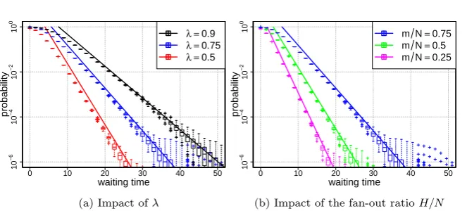
Theorem 6 _{(Random Mapping, Renewals, Non-Blocking)}Given a FJ queueing system withN servers and random partial mapping of jobs toH ≤N

servers based on a uniform distribution over the set{A⊆ {1, . . . , N}||A|=H}

waiting time

probability

λ =0.9

λ =0.75

λ =0.5

0 10 20 30 40 50

10

−6

10

−4

10

−2

10

0

(a) Impact ofλ

waiting time

probability

m N=0.75

m N=0.5

m N=0.25

0 10 20 30 40 50

10

−6

10

−4

10

−2

10

0

(b) Impact of the fan-out ratioH/N

Fig. 8 Bounds on the waiting time distributions vs. simulation box-plots for renewal input with random server mapping. The parameters areN= 16, µ= 1. (a) Here, we fix the fan-out ratio toH = 12 and change the job arrival rateλ∈ {0.5,0.75,0.9}while in (b) we fix the arrival rate toλ= 0.75 and vary the fan-out ratioH/N∈ {0.25,0.5,0.75}. Simulations include 100 runs, each accounting for 106 _slots.

arrivals. If the task service times xn,j are iid, then the steady-state waiting

and response timeswandr are bounded by

P[w≥σ]≤He−θσ ,

P[r≥σ]≤HEeθx1,1_e−θσ _,

whereθ is the solution of

(1−pd) +pdE

eθxn,i_Ee−θt1_{= 1. (39)}

Proof The proof goes along similar steps as for Theorem 5, however, using the process

zn(k) =eθ

Pk

i=1(¯xn,i−ti)

which is a martingale for eachn≤N under the criterion (39) onθ.

Figure 8 shows a numerical illustration of the tightness of the bounds on the waiting time distribution from Theorem 6. The illustrated results are for the example of exponentially distributed interarrival and service times with parametersλandµ, respectively.

By combining the above consideration of the compound service time distri-bution with the results from Section 4, one can extend the analysis of random partial mapping to the case of non-renewal input.

job interarrivals tj as in Section 4, and task service times x¯n,i that are

de-scribed by Eq. (36). Jobs are randomly mapped to servers according to a uni-form distribution over the set of server combinations with cardinalityH. The steady-state waiting and response time distributions are bounded by

P[w≥σ]≤He−θσ ,

P[r≥σ]≤HEeθx1,1_e−θσ _,

whereθ is the solution of

(1−pd) +pdEeθx1,1Λ(θ) = 1.

(Recall thatΛ(θ)was defined as a spectral radius ofTθ in Section 4).

Proof The proof follows analogously to the proof of Theorem 3 with the dif-ference thatxn,i is replaced by ¯xn,i andN byH, respectively.

Remark: Random number of servers H:One variation of the system that is considered in Sect. 5.2 is a random mapping of arriving jobs to a random number of servers 1≤H ≤N based on a uniform distribution over the power set {2A_\

∅} with A={1, . . . , N}. In this case the steady state waiting and

response times are bounded by

P[w≥σ]≤N e−θσ ,

P[r≥σ]≤NE

eθx1,1_e−θσ _,

whereθ is the solution of (39) withpd= 2N−1/(2N−1).

6 Application to Window-based Protocols over Multipath Routing

In this section we slightly adapt and use the non-blocking FJ queueing system from Section 3.1 to analyze the performance of agenericwindow-based trans-mission protocol over multipath routing. While this problem has attracted much interest lately with the emergence of multipath TCP [35], it is subject to a major difficulty due to the likely overtaking of packets on different paths. Consequently, packets have to additionally wait for aresequencing delay, which directly corresponds to the synchronization constraint in FJ systems. We note that the employed FJ non-blocking model is subject to a convenient simplifi-cation, i.e., each path is modelled by a single server/queue only.

paths. We also assume that packets on each path are delivered in a (locally-) FIFO order, i.e., there is no overtaking on the same path.

In analogy to Section 3.1, we consider a batch waiting until its last packet starts being transmitted. When the transmission of the last packet of batch

j begins, the previous batch has already been received, i.e., all packets of the batchj−1 are in order at nodeB.

We are interested in the response times of the batches, which are upper bounded by the largest response time of the packets therein. The arrival time of a batch is defined as the latest arrival time of the packets therein, i.e., when the batch is entirely received. Formally, the response time of batch j∈ {lN+ 1|l∈N}can be given by slightly modifying (2), i.e.,

rj= max

0≤k≤j−1

(

max

n ( k

X

i=0

xn,j−i− k X

i=1 tn,j−i

))

.

The corresponding steady-state response time has the modified representation

r=D max

k≥0

(

max

n ( k

X

i=0 xn,i−

k X

i=1 tn,i

))

.

The modifications account for the fact that the packets of each batch are asyn-chronously transmitted on the corresponding paths (instead, in the basic FJ systems, the tasks of each job are simultaneously mapped). In terms of nota-tions, the tn,i’s now denote the interarrival times of the packets transmitted

over the same pathn, whereasxn,i’s are iid and denote the transmission time

of packet i over path n; as an example, when the arrival flow at node A is Poisson,tn,i has an ErlangEN distribution for allnandi.

We next analyze the performance of the considered multipath routing for both renewal and non-renewal input.

Renewal Arrivals

Consider first the scenario with renewal interarrival times. Similarly to Sec-tion 3.1 we bound the distribuSec-tion of the steady-state response timer using a submartingale in the time domainj ∈ {lN+ 1|l ∈N}. Following the same

steps as in Theorem 1, the process

zn(k) =eθ(

Pk

i=0xn,i−Pki=1tn,i)

is a martingale under the condition

Eeθx1,1_Ee−θt1,1_{= 1 ,}

where we used the filtration

…

.

time

batch

time

batch

A

B

Fig. 9 A schematic description of the window-based transmission over multipath routing; each path is modelled as a single server/queue.

Note that Ee−θt1,1_{denotes the Laplace transform of the interarrival times}

of packets transmitted over each path. The proof that maxnzn(k) is a

sub-martingale follows a similar argument as in (10). Hence, we can bound the distribution of the steady-state response time as

P[r≥σ]≤NE

eθx1,1_e−θσ _{, (40)}

with the condition onθ from above.

Non-Renewal Arrivals

Next, consider a scenario with non-renewal interarrival timestiof the packets

arriving at the fork nodeA in Figure 9, as described in Section 4. On every pathn∈[1, N] the interarrivals are given by a sub-chain (cn,k)kthat is driven

by theN-step transition matrix TN _{= (α}

i,j)i,j forT given in (23). Similarly

as in the proof of Theorem 3, we will use an exponential transform (TN₎ θ of

the transition matrix that describes each pathn, i.e.,

(TN)θ:=

α1,1β1 α1,2β2 α2,1β1 α2,2β2

,

withαi,j defined above andβ1, β2 being the elements of a vectorβ of condi-tional Laplace transforms ofN consecutive interarrival timesti. The vectorβ

is given by

β :=

β1 β2

=



  

Ehe−θPNi=1ti c1= 1

i

Ehe−θPN i=1ti

c1= 2

i 

and can be computed given the transition matrixT from (23) via an exponen-tial row transform [10] (Example 7.2.7) denoted by

˜

Tθ:= 



(1−p)Ee−θL1 _pEe−θL1

qEe−θL2_(1−q)Ee−θL2



 ,

yieldingβ= ( ˜Tθ)N

1 1

.

DenoteΛ(θ) andh= (h(1), h(2)) as the maximal positive eigenvalue of the matrix (TN)θand the corresponding right eigenvector, respectively. Mimicking

the proof of Theorem 3, one can show for every pathnthat the process

zn(k) =h(cn,k)eθ(

Pk

i=0xn,i−Pki=1tn,i)

is a martingale under the condition on (positive)θ

E

eθx1,1_{Λ(θ) = 1. (41)}

Given the martingale representation of the processeszn(k) for every path n, the process

z(k) = max

n zn(k)

is a submartingale following the line of argument in (10). We can now use (30) and the remark at the end of Section 4.1 to bound the distribution of the steady-state response timeras

P[r≥σ]≤ E[h(c1,1)] h(2) NE

eθx1,1_e−θσ _{, (42)}

where we also used thathis monotonically decreasing andθas defined in (41).

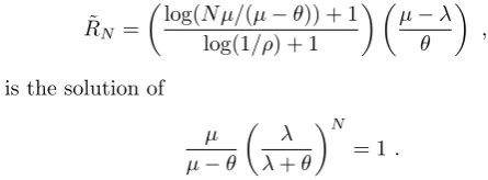
As a direct application of the obtained stochastic bounds (i.e., (40) and (42)), consider the problem of optimizing the number of parallel pathsN sub-ject to the batch delay (accounting for both queueing and resequencing delays). More concretely, we are interested in the number of paths N minimizing the overall average batch delay. Note that the path utilization changes withN as

ρ= λ

N µ ,

since each path only receives _N1 of the input. In other words, the packets on each path are delivered much faster with increasing N, but they are subject to the additional resequencing delay (which increases as logN as shown in Section 3.1).

To visualize the impact of increasing N on the average batch response times we use the ratio

˜

RN := E[rN]

1 2 3 4 5

0.1

1

10

number of paths

R

~ N

ρ =0.5

ρ =0.75

ρ =0.9

(a) Renewal

1 2 3 4 5

0.1

1

10

number of paths

R

~ N

ρ =0.5

ρ =0.75

ρ =0.9

(b) Non-renewal

Fig. 10 Multipath routing reduces the average batch response time when ˜RN<1; smaller

˜

RN corresponds to larger reductions. Baseline parameter µ = 1 and non-renewal

pa-rameters: p = 0.1, q = 0.4, λ1 = {0.39,0.7,0.88}, λ2 = 0.95, yielding the utilizations

ρ={0.5,0.75,0.9}(from top to bottom).

where, with abuse of notation, E[rN] denotes a bound on the average batch

response time for someN, andE[r1] denotes the corresponding baseline bound forN = 1; both bounds are obtained by integrating either (40) or (42) for the renewal and the non-renewal case, respectively.

In the renewal case, with exponentially distributed interarrival times with parameterλ, and homogenous paths/servers where the service times are ex-ponentially distributed with parameterµ, we obtain

˜

RN =

_{log(N µ/(µ−θ)) + 1}

log(1/ρ) + 1

µ−λ θ

, (43)

whereθ is the solution of

µ µ−θ

λ λ+θ

N

= 1 .

In the non-renewal case we obtain the same expression for ˜RN as in (43)

except for the additional prefactor E[h(c1(1))]

h(2) prior to N; moreover, θ is the implicit solution from (41).

Figure 10 illustrates ˜RN as a function ofN for several utilization levelsρ

the technical explanation (in (a)) is that the waiting time in the underlying

EN/M/1 queue quickly converges to _µ1, whereas the resequencing delay grows

as logN; in other words, the gain in the queueing delay due to multipath routing is quickly dominated by the resequencing delay price.

7 Conclusions

In this paper we have provided the first computable and non-asymptotic bounds on the waiting and response time distributions in Fork-Join queue-ing systems under full and partial server mappqueue-ing. We have analyzed four practical scenarios comprising of either workconserving or non-workconserving servers, which are fed by either renewal or non-renewal arrivals. In the case of workconserving servers, we have shown that delays scale as O(logN) in the number of parallel servers N, extending a related scaling result from renewal to non-renewal input. In turn, in the case of non-workconserving servers, we have shown that the same fundamental factor of logNdetermines the system’s stability region. Given their inherent tightness, our results can be directly ap-plied to the dimensioning of Fork-Join systems such as MapReduce clusters and multipath routing. A highlight of our study is that multipath routing is reasonable from a queueing perspective for two routing paths only.

References

1. Amazon Elastic Compute Cloud EC2. http://aws.amazon.com/ec2

2. Abate, J., Choudhury, G.L., Whitt, W.: Exponential approximations for tail probabili-ties in queues, I: Waiting times. Oper. Res.43, 885–901 (1995)

3. Babu, S.: Towards automatic optimization of MapReduce programs. In: Proc. of ACM SoCC, pp. 137–142 (2010)

4. Baccelli, F., Gelenbe, E., Plateau, B.: An end-to-end approach to the resequencing problem. J. ACM31(3), 474–485 (1984)

5. Baccelli, F., Makowski, A.M., Shwartz, A.: The Fork-Join queue and related systems with synchronization constraints: Stochastic ordering and computable bounds. Adv. in Appl. Probab.21(3), 629–660 (1989)

6. Balsamo, S., Donatiello, L., Van Dijk, N.M.: Bound performance models of heteroge-neous parallel processing systems. IEEE Trans. Parallel Distrib. Syst.9(10), 1041–1056 (1998)

7. Billingsley, P.: Probability and Measure, 3rd edn. Wiley (1995)

8. Boxma, O., Koole, G., Liu, Z.: Queueing-theoretic solution methods for models of par-allel and distributed systems. In: Proc. of Performance Evaluation of Parallel and Distributed Systems. CWI Tract 105, pp. 1–24 (1994)

9. Buffet, E., Duffield, N.G.: Exponential upper bounds via martingales for multiplexers with Markovian arrivals. J. Appl. Probab.31(4), 1049–1060 (1994)

10. Chang, C.S.: Performance Guarantees in Communication Networks. Springer (2000) 11. Chen, Y., Alspaugh, S., Katz, R.: Interactive analytical processing in big data systems:

A cross-industry study of mapreduce workloads. Proc. VLDB Endow.5(12), 1802–1813 (2012)

12. Ciucu, F., Poloczek, F., Schmitt, J.: Sharp per-flow delay bounds for bursty arrivals: The case of FIFO, SP, and EDF scheduling. In: Proc. of IEEE INFOCOM, pp. 1896–1904 (2014)

14. Duffield, N.: Exponential bounds for queues with Markovian arrivals. Queueing Syst.

17(3–4), 413–430 (1994)

15. Flatto, L., Hahn, S.: Two parallel queues created by arrivals with two demands I. SIAM J. Appl. Math.44(5), 1041–1053 (1984)

16. Ganesh, A., O’Connell, N., Wischik, D.: Big queues. No. 1838 in Lecture notes in mathematics. Springer (2004)

17. Gibbens, R.J.: Traffic characterisation and effective bandwidths for broadband network traces. J. R. Stat. Soc. Ser. B. Stat. Methodol. (1996)

18. Han, Y., Makowski, A.: Resequencing delays under multipath routing - Asymptotics in a simple queueing model. In: Proc. of IEEE INFOCOM, pp. 1–12 (2006)

19. Harrus, G., Plateau, B.: Queueing analysis of a reordering issue. IEEE Trans. Softw. Eng.8(2), 113–123 (1982)

20. Jiang, Y., Liu, Y.: Stochastic Network Calculus. Springer (2008)

21. Joshi, G., Liu, Y., Soljanin, E.: Coding for fast content download. In: Proc. of the Allerton Conference on Communication, Control, and Computing, pp. 326–333 (2012) 22. Joshi, G., Liu, Y., Soljanin, E.: On the delay-storage trade-off in content download from

coded distributed storage systems. IEEE J. Sel. Areas Commun.32(5), 989–997 (2014) 23. Kandula, S., Sengupta, S., Greenberg, A., Patel, P., Chaiken, R.: The nature of data center traffic: Measurements & analysis. In: Proc. of ACM IMC, pp. 202–208 (2009) 24. Kavulya, S., Tan, J., Gandhi, R., Narasimhan, P.: An analysis of traces from a

produc-tion MapReduce cluster. In: Proc. of IEEE/ACM CCGRID, pp. 94–103 (2010) 25. Kemper, B., Mandjes, M.: Mean sojourn times in two-queue Fork-Join systems: Bounds

and approximations. OR Spectr.34(3), 723–742 (2012)

26. Kesidis, G., Urgaonkar, B., Shan, Y., Kamarava, S., Liebeherr, J.: Network calculus for parallel processing. In: Proc. of the ACM MAMA workshop (2015)

27. Kingman, J.F.C.: Inequalities in the theory of queues. J. R. Stat. Soc. Ser. B. Stat. Methodol.32(1), 102–110 (1970)

28. Ko, S.S., Serfozo, R.F.: Sojourn times in G/M/1 Fork-Join networks. Naval Res. Logist.

55(5), 432–443 (2008)

29. Lebrecht, A.S., Knottenbelt, W.J.: Response time approximations in Fork-Join queues. In: Proc. of UKPEW (2007)

30. Lu, H., Pang, G.: Gaussian limits for a Fork-Join network with nonexchangeable syn-chronization in heavy traffic. Math. Oper. Res.41(2), 560–595 (2016)

31. Nelson, R., Tantawi, A.: Approximate analysis of Fork/Join synchronization in parallel queues. IEEE Trans. Computers37(6), 739–743 (1988)

32. Pike, R., Dorward, S., Griesemer, R., Quinlan, S.: Interpreting the data: Parallel analysis with Sawzall. Sci. Program.13(4), 277–298 (2005)

33. Polato, I., R, R., Goldman, A., Kon, F.: A comprehensive view of Hadoop research - a systematic literature review. J. Netw. Comput. Appl.46(0), 1 – 25 (2014)

34. Poloczek, F., Ciucu, F.: Scheduling analysis with martingales. Perform. Evaluation79, 56–72 (2014)

35. Raiciu, C., Barre, S., Pluntke, C., Greenhalgh, A., Wischik, D., Handley, M.: Improving datacenter performance and robustness with multipath TCP. SIGCOMM Comput. Commun. Rev.41(4), 266–277 (2011)

36. R´enyi., A.: On the theory of order statistics. Acta Math. Hungar. 4(3–4), 191–231 (1953)

37. Tan, J., Meng, X., Zhang, L.: Delay tails in MapReduce scheduling. SIGMETRICS Perform. Eval. Rev.40(1), 5–16 (2012)

38. Tan, J., Wang, Y., Yu, W., Zhang, L.: Non-work-conserving effects in MapReduce: Diffusion limit and criticality. SIGMETRICS Perform. Eval. Rev.42(1), 181–192 (2014) 39. Varki, E.: Mean value technique for closed Fork-Join networks. SIGMETRICS Perform.

Eval. Rev.27(1), 103–112 (1999)

40. Varma, S., Makowski, A.M.: Interpolation approximations for symmetric Fork-Join queues. Perform. Evaluation20(1–3), 245–265 (1994)

41. Vianna, E., Comarela, G., Pontes, T., Almeida, J., Almeida, V., Wilkinson, K., Kuno, H., Dayal, U.: Analytical performance models for MapReduce workloads. Int. J. Parallel Prog.41(4), 495–525 (2013)

43. Xia, Y., Tse, D.: On the large deviation of resequencing queue size: 2-M/M/1 case. IEEE Trans. Inf. Theory54(9), 4107–4118 (2008)

44. Zaharia, M., Konwinski, A., Joseph, A.D., Katz, R., Stoica, I.: Improving MapReduce performance in heterogeneous environments. In: Proc. of USENIX OSDI, pp. 29–42 (2008)

Appendix

We assume throughout the paper that all probabilistic objects are defined on a common filtered probability space Ω,A,(Fn)n,P

. All processes (Xn)nare assumed to beadapted,

i.e., for eachn≥0, the random variableXnisFn-measurable.

Definition 1 (Martingale) An integrable process (Xn)nis amartingaleif and only if for

eachn≥1

E[Xn| Fn−1] =Xn−1 . (44)

Further,Xis said to be a sub-(super-)martingale if in (44) we have≥(≤) instead of equality.

The key property of (sub, super)-martingales that we use in this paper is described by the following lemma:

Lemma 1 (Optional Sampling Theorem) Let(Xn)nbe a martingale, andKa bounded

stopping time, i.e.,K≤na.s. for somen≥0and{K=k} ∈ Fkfor allk≤n. Then

E[X0] =E[XK] =E[Xn] . (45)

IfX is a sub-(super)-martingale, the equality sign in (45) is replaced by≤(≥).

Proof See, e.g., [7].

Note that for any(possibly unbounded) stopping timeK, the stopping timeK∧nis always bounded. We use Lemma 1 with the stopping timesK∧nin the proofs of Theorems 1 – 4.

Lemma 2 Letck be the Markov chain from Figure 4 andK be the stopping time from

(11). Then the distribution of(cK|K <∞)is stochastically smaller than the steady-state

distribution ofck, i.e.,

P[cK= 2|K <∞]≤P[c1= 2] ,

or, equivalently,

E[h(cK)|K <∞]≥E[h(ck)] ,

for all monotonically decreasing functionshon{1,2}.

Proof Using Bayes’ rule and the stationarity of the processck, it holds:

P[cK = 2|K <∞] =

∞

X

k=1

P[ck= 2|K=k]P[K=k]

=

∞

X

k=1

P[K=k|ck= 2]P[ck= 2]

=P[c1= 2]

∞

X

k=1

SinceL1is stochastically smaller thanL2, we have for anyk≥1

P[K=k|ck= 2]

=P

" tk≤max

n k

X

i=1

xn,i− k−1

X

i=1

ti−σ,max n

k−1

X

i=1

(xn,i−ti)< σ

ck= 2

#

≤P

" tk≤max

n k

X

i=1

xn,i− k−1

X

i=1

ti−σ,max n

k−1

X

i=1

(xn,i−ti)< σ

#

=P[K=k] .

HenceP∞