Determining cluster cluster aggregation rate kernals using inverse methods

(1)

University of Warwick institutional repository: http://go.warwick.ac.uk/wrap

A Thesis Submitted for the Degree of PhD at the University of Warwick

http://go.warwick.ac.uk/wrap/57480

This thesis is made available online and is protected by original copyright.

Please scroll down to view the document itself.

(2)

AUTHOR:Peter P. Jones DEGREE:Ph.D.

TITLE:Determining Cluster-Cluster Aggregation

Rate Kernels Using Inverse Methods

DATE OF DEPOSIT: . . . .

I agree that this thesis shall be available in accordance with the regulations governing the University of Warwick theses.

I agree that the summary of this thesis may be submitted for publication.

Iagreethat the thesis may be photocopied (single copies for study purposes only).

Theses with no restriction on photocopying will also be made available to the British Library for microfilming. The British Library may supply copies to individuals or libraries. subject to a statement from them that the copy is supplied for non-publishing purposes. All copies supplied by the British Library will carry the following statement:

“Attention is drawn to the fact that the copyright of this thesis rests with its author. This copy of the thesis has been supplied on the condition that anyone who consults it is understood to recognise that its copyright rests with its author and that no quota-tion from the thesis and no informaquota-tion derived from it may be published without the author’s written consent.”

AUTHOR’S SIGNATURE: . . . .

USER’S DECLARATION

1. I undertake not to quote or make use of any information from this thesis without making acknowledgement to the author.

2. I further undertake to allow no-one else to use this thesis while it is in my care.

DATE SIGNATURE ADDRESS

. . . .

(3)

Determining Cluster-Cluster Aggregation

Rate Kernels Using Inverse Methods

by

Peter P. Jones

Thesis

Submitted to the University of Warwick

for the degree of

Doctor of Philosophy

(4)

List of Figures

2.1 Example scaling distribution . . . 13

2.2 Example local regime stationary distribution . . . 17

2.3 Example growing stationary distribution . . . 19

3.1 Gillespie Monte Carlo simulation optimisation pattern. . . 26

3.2 Monte Carlo simulation calibration: scaling distributions . . . 29

3.3 Monte Carlo simulation calibration: stationary distributions . . . 32

3.4 Collective oscillations around stationary state attractors . . . 34

3.5 Site total massM1(t)time series exhibiting quasicycles. . . 39

3.6 Site total mass autocorrelation functions . . . 41

4.1 Inversions from Monte Carlo data: constant and sum kernels . . . 56

4.2 Inversions from Monte Carlo data: fractional homogeneity sum kernels . . 57

4.3 Optimal representation error: fractional exponent sum kernels . . . 59

5.1 Example factorised kernel shape functions . . . 66

5.2 Example scaling decay case distribution: Sum kernel withλ=0.5 . . . 71

5.3 Fourier series estimations of selected shape functions . . . 76

5.4 Reproduced stationary distributions . . . 77

(8)

5.6 Saturn’s Rings kernel estimation . . . 78

5.7 Generalised Brownian Coagulation kernel estimations. . . 80

5.8 Differential Sedimentation kernel estimation . . . 81

5.9 Estimated decay case sum kernels . . . 83

5.10 Estimated ‘van Dongen’ form kernels . . . 85

(9)

List of Tables

(10)

Acknowledgments

I would like to express profound gratitude to the following entities and individuals. To the

EPSRC for the funding, and to the University of Warwick for being a wonderful institution.

To Prof. Robin Ball, for the initial opportunity and ongoing support of the project. To

Dr. Colm Connaughton for the excellent guidance and support provided throughout. To the

remarkable Complexity Science DTC administrators, Phil Richardson, Monica Lucena, and

Jen Bowskill, who made everything seem so seamless on the surface. Especially to Monica,

who helped to smooth out the first few years of the ups and downs of the PhD process with a

unique mixture of spirit and magnanimity. To friends, colleagues, and staff in the DTC and

the Warwick Maths Institute, for being brilliant. To my family, for always being there. To

anyone else who made the slightest contribution to helping this project along. Many thanks

(11)

Declarations

To the best of this author’s knowledge the text of this thesis is entirely the work of its

author except where otherwise indicated. The following are precise attributions regarding

thesis content, including references to earlier texts by the author.

• Some text in the abstract and introductory chapter may have appeared earlier on the

author’s university webpage, in the online document “Determining Cluster-Cluster

Aggregation Rate Kernels Using Inverse Methods: A Brief Non–mathematical

In-troduction to this Research for the Uninitiated” available via that webpage, and in

contributions to prior papers mentioned below. At the time of thesis publication the

webpage is at

http://www2.warwick.ac.uk/fac/cross_fac/complexity/people/students/dtc/students2007/peterjones

• The incidental discovery (mentioned in Chapter3), that significant oscillations persist

in the presence of noise under certain nonlocal parameterisations of the finite size

aggregation problem with source, was made by the author during the course of this

research. It was investigated further in the multi-author paper (led by Connaughton)

published asBall et al.[2012].

• During this research, the author also made the incidental discovery (also mentioned in

Chapter3) that for certain finite system size Monte Carlo integrations of the

aggrega-tion problem with source the staaggrega-tionary distribuaggrega-tion in the nonlocal regime perturbed

(12)

• The initial sets of exact distribution data used during the research in Chapter4were

supplied by Connaughton.

• The paperConnaughton and Jones [2011] was based upon the work undertaken in

Chapter4.

• The novel regularisation function used inConnaughton and Jones [2011] and

men-tioned in Chapter4was discovered by the author.

• The novel inverse method in Chapter5is a joint construction by Ball, Connaughton,

and the author. The research investigating the actual properties of the method, and

the refinements and adaptations resulting therefrom are the work of this author. At

the time of writing, a preprint paper based on the work is available at

(13)

Abstract

(14)

Chapter 1

Introduction

1.1 Prelude

An inverse problem is usually the data-driven complement of an existing theoretical

for-ward problem. In a forfor-ward problem, we have investigated a physical phenomenon that

we think we have a good theoretical model for, and have obtained experimental data. The

task is to implement the model, compare the data that it produces with the experimental

data, and to explain the differences, if any. With an inverse problem typically there is only

a rough idea of what the model should be for some given phenomenon, and values of key

parameters in the model are unknown. Given experimental data for the real phenomenon,

the inverse problem is the attempt to determine the values of the key model parameters from

the data1. If the data is sufficiently complete this task is relatively easy. But if the data is

sparse or contains noise, then matters become more difficult.

1_{Asserting that there is a real distinction between inverse problems and parameter estimation problems}

(15)

In this thesis we deal specifically with a class of inverse problems concerning

cluster-cluster aggregation (CCA). A basic description of the process involved in CCA is given by

the following case. Imagine some oil mixed with water; two liquids that are immiscible in

the same container. Also imagine that the mixture has been thoroughly stirred so that there

are many very small globules of oil, of roughly equal size, evenly distributed throughout the

water. Then we leave the mixture alone, and allow the currents within the fluid to bring oil

globules together here and there as time passes. Typically, when two oil globules of masses

m1 andm2 come into contact with each other they will merge to form a larger globule of

massm=m1+m2. Mass is conserved in this merger process, so the mass of the large

globule is equal to the sum of the masses of the two contributing globules.

For such a system the total pattern of mergers can be considered to be physically

ir-reversible, in the sense that the likelihood of the large globule of massm spontaneously

decomposing into two globules with precisely the massesm1 andm2 at some future time

(before other events overtake matters) is small, and for the entire system of mergers, the

entire reverse process that returns everything to its initial conditions has infinitesimal

like-lihood. In broad physical terms, these small probabilities of the reversal are because some

kinetic or potential energy is dissipated during the process of aggregation and at the

mi-croscale the space of configurations is huge and changing, so the chances of energy being

returned in precisely the way needed to reverse the aggregation neatly are very slight (and

may even be zero). Types of system where irreversible bonding is a physical fact are

obvi-ously irreversible in this way.

In other aggregation processes the masses might also have geometric structure, like grains

of sand, molecules or pollen, and instead of merging into a bigger blob, they aggregate to

form larger clusters with spatial structure. Clusters can, of course, aggregate with other

(16)

overlook this should we choose to if we can argue for deliberately making some averaging

approximation to simplify our models. If this is done, then we could treat the clusters as

being effectively pointlike with all the details of geometry being averaged away. This is one

aspect that distinguishes the process of cluster-cluster aggregation (CCA) from, for

exam-ple, diffusion limited aggregation (DLA). (In DLA the object of study is the formation of a

cluster from the accumulation of lone small masses over time - e.g. water molecules joining

a snowflake under freezing conditions - and the study of the resulting cluster structures is a

prominent concern.)

We might also imagine that the process of merger between globules could happen

(sta-tistically, averaging over a large number of mergers) at a rate dependent on the magnitudes

of two contributing masses. For example, if there is a very large globule in a sea of very

small globules then we might expect mergers between the large globule and small globules

to happen at a faster rate than mergers between small globules, simply because the large

globule occupies more space and constitutes a bigger target as the mixture swirls.

How-ever, in another completely different mixture, mergers between large and small globules

might be less likely, and hence happen at a slower rate, because of chemical, electrostatic,

or hydrodynamic interferences.

Research in cluster-cluster aggregation has progressed for a long time using a model

based on the Smoluchowski Coagulation Equation (SCE) [Smoluchowski, 1917]. It has

been used to successfully model aggregation, coagulation, and coalescence processes that

abound in nature and span all scales, ranging from the microscopic scales of atmospheric

aerosol formation [Friedlander,1977], to the cosmological scales of the clustering of

mat-ter within the universe [Silk and White, 1978]. The effectiveness of the SCE relies on

(17)

wise interactions between particles are likely. That is, the SCE states that the mean number

of massesN(m,t) (per unit of volume) of massm present at some timet, averaged over

suitably sized regions within the mixture, is a function of the similarly spatially-averaged

rates at which other pairs of masses present can clump together to form a mass of sizem,

minus the spatially-averaged rates at which masses of sizemmight join with other masses.

Our ability to apply averaging assumptions to the problem places the SCE in the class of

so-called mean-field approximations, which are valid only if we can average over a

suffi-ciently large number of interactions to be able to talk sensibly about the changes in number

densityN(m,t)being independent from spatial correlations. This translates into being able

to assume that the density of pairs of masses factorises at all timest>0, such that,

N(2)(m1,m2,t)∝N(m1,t)N(m2,t) (1.1)

Under this mean-field assumption, the system of equations represented by the SCE

ex-hibits closure, with changes in concentrations depending only upon other concentrations

(first-order densities) and not upon an entire hierarchy of product density functions,

N(2)(m₁,m₂,t),N(3)(m₁,m₂,m₃,t), ..., (1.2)

An advantage of the SCE is that it is the simplest effective description of an aggregating

system. However, there are also some snags with the SCE. One is that many real systems are

not vast and internally they exhibit (statistical) spatial heterogeneities - for example if large

masses hoover up all smaller masses in their immediate neighbourhood creating ‘moats’ of

empty liquid around them - so the averaging can break down. Another snag is that even in

(18)

of injected mass, analytic solutions for the evolution of the distributions of mass sizes over

time are known for only a few special aggregation rate kernel functions. Hence, in general,

there is both the forward problem of predicting the likely outcome of using some other

kernel function in some process, and the inverse problem of inferring kernels from observed

data for the mass (density) distributionN(m,t). Computer simulations of aggregation can

be made for specific forward problems, but it is excessively time-consuming to attempt to

find which kernel matches a particular mass distribution by simulating all parameterisations

of some subset of all classes of possible kernels. Hence the efforts to find effective, efficient

inverse methods.

1.2 The Contemporary Relevance of the Inverse Problem

A particular example that is of strong contemporary interest is the role played by droplet

coalescence in cloud formation and the clouds’ internal dynamics. A better understanding

of this process would improve the precision of climate evolution projections [Stephens,

2005].

However, considering real aggregation systems like the formation of raindrops,

turbu-lence in the supporting medium (the cloud air mass) complicates the task significantly. It

may have a non-trivial role in determining the collision rate of water droplets [Bodenschatz

et al.,2010][Grabowski and Wang,2009]. Moreover, it seems likely that turbulence at larger

scales interacts strongly with the micro-physics of the rain formation process. Coupling

the macro- and microscopic scales of simulation of weather systems remains a significant

computational challenge. While small-volume direct numerical simulation of droplets in

turbulent flows [Reade and Collins,2000][Wang et al.,2008] are possible, it is not yet clear

(19)

Complete theoretical description of the statistical interplay between particles and

tur-bulence also remains elusive. However, owing to recent technological advances, both the

quality and quantity of empirical data obtained from observations have significantly

in-creased [Siebert et al., 2006]. It therefore makes sense to explore using inverse methods

upon this data as means to obtain useful insights. The use of inverse methods can also

provide additional quantitative measures for optimising the choice of model in contexts in

which the microphysics is unknown or controversial.

The inverse problem which we discuss in this thesis is to extract the functional form

of the mass-dependent coalescence rates2,K(m₁,m₂), given the measurements of the time

evolution of the droplet size distribution,N(m,t). Prior methods for this problem are found

inWright and Ramkrishna[1992] andOnishi et al.[2011]. (Wright and Ramkrishna[1992]

is the most general development from precursors in Muralidhar and Ramkrishna[1986],

Muralidhar and Ramkrishna [1989], Wright et al. [1990], Wright et al. [1992]. Onishi

et al. [2011] extends developments inOnishi et al. [2008].) In Onishi et al. [2011] the

method does not depend upon self-similarity of N(m,t) but significant prior knowledge

about droplet coalescence in turbulent conditions was used to put strong constraints on the

functional form of the kernel, thus simplifying the inversion problem at the expense of a

loss of generality. The method inWright and Ramkrishna[1992], for use with self-similar

decay case distributions, does not strongly constrain the kernel form, but the paper only

treated example kernels with homogeneity exponents3,λ ∈ {0,1}.

In this thesis we demonstrate that a weakness of the Wright and Ramkrishna [1992]

method is that it does not retrieve kernel functions containing fractional order exponents

sufficiently well. We then provide a new inverse method which assumes only kernel

homo-geneity and yet exhibits powerful new capabilities in respect of the inverse problem under

2_{For its mathematical role within the SCE this function is also called a kernel function.}

3_{See equation (}_2.5_{) for the definition of the kernel homogeneity exponent}

(20)

consideration. For a broad class of kernel functions, we demonstrate that our method will

retrieve good representations of kernels from the main forms of distribution data. (See

Chapter2for more details about the forms of mass distributions, and AppendixBfor some

information about the kernel functions we used to generate test data sets).

1.3 Thesis Structure

In Chapter2, the properties of the SCE are introduced, and we provide a brief overview of

the different classes of solutions. Then in Chapter3 simulation of the SCE using Monte

Carlo techniques is discussed, and some incidental discoveries made using the Monte Carlo

simulations are mentioned. The main research material is then presented in two subsequent

chapters. Chapter4(see alsoConnaughton and Jones[2011]) investigates the capacity of

method in Wright and Ramkrishna [1992] in respect of concerns about fractional order

kernel exponents. In Chapter 5 we propose a novel and more powerful method whose

properties are assessed in respect of the main forms ofN(m,t)mass distribution data.

1.4 A Note on Terminology

Throughout this thesis we will use the following (non-standard) terminological

short-hand. When we refer to thedecay casewe mean a system that has an initial mass

distri-bution,N(m,0), but no constant source of injected mass. The system then evolves through

aggregations taking place, and the mass distributionN(m,t) “decays” until a single large

mass remains. In the literature the decay case is usually described as “aggregation without

source”. Calling it the decay case in the text makes it easier to distinguish from the classes

(21)

Chapter 2

Cluster-Cluster Aggregation and the

Smoluchowski Coagulation Equation

2.1 General Properties

For a large variety of aggregation phenomena the Smoluchowski Coagulation Equation

(SCE) [Smoluchowski,1917] gives a mean-field description of the evolution of the average

concentrations,N(m,t), of mass sizes mper unit volume in a suitably large, dilute, and

well-mixed, system of coalescing or aggregating masses in some supporting medium. A

good example is chemical monomers with suitable bonding properties in suspension. The

individual masses diffuse or are advected within the fluid and they collide, sticking together

with some probability.

With respect to the study of clouds the utility of the SCE lies in approximating

phenom-ena such as the formation of rain from smaller water droplets [Rogers and Yau,1989], or

study of the coagulation of dust or soot particles [Friedlander,1977], such as those ejected

into the atmosphere from desert winds, volcanic eruptions [Costa et al., 2010] or

(22)

thought to play a role in the rate of formation of rain [Falkovich et al., 2002] (though the

degree of influence remains a matter of some debate [Devenish et al.,2012]), and there is

an analog of the SCE for the cascades of energy between different scales of turbulent eddies

[Connaughton et al.,2006]. So the SCE would perhaps be expected to play a significant

role in modelling droplet coagulation in a turbulent medium during the formation of rain.

Mathematically and in numerical simulation, the SCE can be approached as a

determinis-tic system of integro-differential equations, or treated probabilisdeterminis-tically as a Markov Process

[Aldous, 1999][Bertoin,2006]. We will not discuss the contents of the extensive

proba-bilistic literature in detail here, except to mention the relevance of probaproba-bilistic theorems

concerning convergence toward the mean-field solutions when considering the evolution of

finite mass Monte Carlo simulations [Fournier and Giet,2004] (see also Chapter3).

In the discrete form of the SCE, all larger masses are taken to be multiples of a minimum

(monomer) massm0, and by assuming a convenient rescaling we can takem0=1. The SCE

asserts that the rate of change of the concentration,Nm(t) =N(m,t), for anym∈N, evolves

according to:

∂N(m,t)

∂t = 1 2

m−1

∑

m1=1

K(m−m1,m1)Nm−m1(t)Nm1(t) (2.1)

− ∞

∑

m1=1

K(m,m₁)Nm(t)Nm1(t) +Jδ(m−1)

The first sum on the right hand side of (2.1) represents the total rate at which two smaller

mass combine to form masses of sizem. The second sum represents the total rate at which

masses of sizemcombine with other masses to make masses larger than sizem. Typically,

(23)

average rates at which two massesm1andm2could meet and coalesce. In the decay case of

aggregation without a constant source of injected mass, the rate of mass injection isJ=0.

When there is a source injecting mass into the system, thenJ>0.

For systems constrained to have a finite spectrum of mass sizes the upper limit on the

second sum can be a finite maximum mass size M<∞. Even if the upper limit of the

second sum term is less than infinity, such a finite mass size version of the discrete SCE can

remain valid as a mean-field approximation to that system, assuming an absence of spatial

correlations (on the relevant timescale of observation). Extra terms can be added to such

versions of the SCE depending on whether the masses larger thanM are counted within

total mass conservation, or lost outside the system. IfLM(m)represents the masses larger

thanMone can write,

∂N(m,t)

∂t = 1 2

m−1

∑

m1=1

K(m−m1,m1)Nm−m1(t)Nm1(t) (2.2)

− M−m

∑

m1=1

K(m,m1)Nm(t)Nm1(t) +Jδ(m−1)−LM(m,t)

LM(m,t) = M

∑

m1=M−m+1

K(m,m1)Nm(t)Nm1(t) (2.3)

Irrespective of whether the system has an upper mass size limit or not, when the mass

spectrum is continuous, then the SCE has an equivalent continuous form (sometimes

at-tributed toM¨uller[1928]) as shown in (2.4). In this case there can be interesting discussions

in mathematical treatments about how smallm0must be (see, for example, the discussion

(24)

∂N(m,t)

∂t = 1 2

Z m

0

K(m−m1,m1)N(m−m1,t)N(m1,t)dm1 (2.4)

− Z ∞

0

K(m,m1)N(m,t)N(m1,t)dm1+ J

m₀δ(m−m0)

The assumption of the lack of spatial correlations, averaged over an appropriate timescale,

is the basis for the SCE’s mean-field validity. This spatial homogeneity means that in

sys-tems where the rates of transport, or of collisions, are presumed to be sufficient to overcome

prolonged spatial inhomogeneities, a single point average is effectively representative of the

entire system. Hence the lack of spatial parameters in (2.1) and (2.4).

In the basic case, aggregation is assumed to be irreversible and aggregates do not

frag-ment. Given some initial mass distribution,N(m0,0), and a particular (bounded) function

forK(m1,m2), the SCE provides the evolution of the mass distributionN(m,t)for all mass

sizesmfor timest>0.

2.2 Decay Case Distributions

Decay case distributions are those where an initial input of masses, N(m0,0), at time

t=0 is then allowed to evolve without there being further injections of mass. In the

sub-gelation regime (discussed briefly later in§2.2.2), given a finite initial inputN(m₀,0) =I₀

the system will evolve over time to a single largest massM=I₀. Even in the comparatively

simple decay case, analytic solutions of the SCE forN(m,t) are known only for a limited

set of kernels, including the classic set K(m1,m2)∈ {1,m1+m2,m1m2} (see Krapivsky

et al.[2010],Davies et al. [1999],Wattis [2006], Leyvraz[2003] and references therein)

(25)

On the positive side, since the analytic solutions for the classical cases K(m1,m2) ∈

{1,m₁+m₂,m₁m₂}are known, these can be used to calibrate numerical simulations of the

SCE (see Chapter3). A list of the (discrete and continuous) solutions for these classical

kernels can be found in [Aldous,1999, Table 2]. Modern derivations of these solutions (for

the discrete SCE) found using generating functions can be found inKrapivsky et al.[2010]

andWattis[2006]. For the continuous SCE, the generating functions are replaced by their

continuous counterpart, the Laplace transform.

Considering the decay case for arbitrary kernels, while it is known that for suitable initial

conditions the SCE has a unique solution, it has also been shown that in general (for any

possible initial conditions) solutions of the SCE need not be unique for a given kernel

[Norris,1999]. Even if a single kernel functionK(m₁,m₂) is capable of producing more

than one consistent solution, then this still might not present a problem when inverting

from data to determine the kernel. What matters for the purposes of the inverse problem is

whether a given distributionN(m,t)has a unique kernel, and because the mean-field SCE

is a deterministic differential equation this is true, provided one can make assumptions that

the spread of possible initial conditions is not too broad.

A key consideration that can help to constrain the breadth of the class of initial

condi-tions, is to restrict discussion to the class of physically feasible aggregations. It has been

suggested that kernel functions of physical interest are typically homogeneous functions

of their arguments [Kang et al.,1986]. This is because more realistic kernels often yield

homogeneous kernels in particular limits.

(26)

0.0 0.5 1.0 1.5 _log(m)2.0 2.5 3.0 3.5 4.0 −4 −2 0 2 4 6 8 10 12 log (N (m ))

−1.0 −0.5 _log(m/s(t))0.0 0.5 1.0

[image:26.595.132.495.108.245.2]

−1 0 1 2 3 4 5 6 log (N (m , t) s(t ) 2)

Figure 2.1: The left image shows the evolution in time of the mass distribution for the constant kernelK=1 which has degree of homogeneityλ =0. Each curve is an average from 10 runs simulated using the Monte Carlo method for discrete mass with a maximum mass size cutoff ofM=300. The lines shown are solely for illustrative purposes. The fluctuations as log(m)increases are partly the result of low concentrations of large masses in a system of this size, and partly because of masses larger thanM=300 leaving the system. The right image shows the result of applying rescaling to produce the time-independent scaling distribution.

K(hm1,hm2) =hλK(m1,m2) (2.5)

2.2.1 Scaling Decay Case Distributions

For most homogeneous kernels, the evolution of the mass distribution is typically

self-similar and scaling arguments forN(m,t), as reviewed inLeyvraz[2003], can also be

ap-plied to create some mathematical simplification by mappingN(m,·)→Φ(z), withΦ(z)

being a time-independent distribution curve, as shown in Figure2.1. The mapping takes the

form,

(27)

wheres(t)is the typical cluster size. This can be defined as a ratio of moments of the size

distribution [Leyvraz,2003][Wright and Ramkrishna,1992]. The moments are defined as:

Mn(t) = Z ∞

0

mnN(m,t)dm (2.7)

Then, provided mass is conserved during the evolution of the system, the following

equation provides a valid way to extract the evolution of the scaling typical mass from the

distribution data.

s(t) = M2(t) M1(t)

(2.8)

Knowledge ofs(t) can then be used to obtain the scaling function,Φ(z). As it is

time-invariant,Φ(z)can be considered to determine the shape of the mass distribution.

For decay case systems it can be shown that τ =2 as long as the second moment of

the systemM2 <∞for all times (see e.g. van Dongen and Ernst[1988]). Although the

scaling function is not fully understood it is known that the largezbehaviour is of the form

Φ(z)∼e−βz [Krapivsky et al., 2010, p.155] and in some cases, for practical purposes, it

is considered to be well matched in that regime by a sum of Gamma distributions [Wright

and Ramkrishna,1992][Goodisman and Chaiken,2006]. However, for some kernels this is

not true, and for the purposes of obtaining a suitably continuous function to use in

inver-sion, resorting to approximation using (automated fitting of) piecewise interpolations can

be necessary.

Scaling (or self-similar) solutions for the classical kernels are also known [Connaughton

(28)

[Menon and Pego, 2008], and a great deal is known about the scaling solutions for

ho-mogeneous kernels in general [van Dongen and Ernst,1988][Davies et al.,1999][Leyvraz,

2003][Fournier and Laurenc¸ot,2005][Goodisman and Chaiken,2006]. Scaling arguments

allow for the deduction of properties (typically information about the values of key

expo-nents) of general solutions to the SCE at large times and large masses [van Dongen and

Ernst,1988][Leyvraz,2003]. Usually the scaling limit is defined to be the set of conditions:

t→∞,m→∞but with the ratiom/s(t)kept fixed and finite.

As noted inLeyvraz[2003] the range of solutions to which these arguments apply

de-pends on subtleties of how one defines scaling, with strong or weak notions of convergence.

The mathematical existence of a large class of scaling solutions is shown inFournier and

Laurenc¸ot [2005]. A counter to the problem of broad initial conditions follows for the

classical kernelsK(m1,m2)∈ {1,m1+m2,m1m2}from proof that solutions with

exponen-tial tails attract all solutions with finite(λ+1)th moment [Menon and Pego,2004] in the

regime of large times required by scaling arguments. InLeyvraz[2003] it is asserted that for

a suitable notion ofweak convergence, scaling of the solution holds ‘under all reasonable

circumstances’ (i.e. the class of initial conditions is adequately broad).

Scaling distributions have an obvious advantage over the time–dependent distributions

in that only a few time snapshots are required to demonstrate that scaling is applicable,

and hence the data collection requirements are more in alignment with contemporary real

collection capabilities. Since the homogeneous kernels that give rise to scaling solutions

are also time-independent functions, scaling distributions still contain enough information

to enable inference of key kernel properties. Although for finite size systems the scaling

hypothesis only holds approximately, in many cases the rescaling collapse approximates a

(29)

2.2.2 Gelation

It can be demonstrated that for infinite systems and homogeneous kernels with λ ≥1

(e.g.K(m₁,m₂) =m₁m₂) that the aggregating system will undergo a transition called

gela-tion within a finite time. At the critical timetc <∞the second moment of the mass

dis-tribution diverges. It can even happen thattc=0 in the instantaneously gelling case. An

interpretation of this is that a single mass (called the gel) of infinite size is formed. See

Krapivsky et al.[2010] for an introduction to these issues,Lushnikov[2006] for a review

with a probabilistic viewpoint, andBall et al.[2011] for an insightful contemporary update

especially concerning finite system size effects, and the references therein.

Since treatment of the inverse problem for decay case systems with gelation is beyond

the scope of this thesis, we will not discuss those further here. However, our new inversion

method presented in Chapter5does treat the finite mass spectrum stationary distributions

for kernels that would be gelling kernels in the infinite mass spectrum decay case.

2.3 Stationary Distributions

Stationary distributions arise when there is a constant injection of small masses into the

system, withJ>0 (typically normalised to beJ=1), and a finite upper mass size cutoff,

M, beyond which masses leave the system. Under these conditions, eventually the rate of

change of the concentrations tends to zero,∂tN(m,t) =0, and the solution of the SCE is

time-independent, asN(m).

2.3.1 Local and Nonlocal Regimes

Before discussing the forms of distributions it is worth noting that in the theoretical

(30)

µ+ν=λ [van Dongen and Ernst,1988][Lee,2000], whereµ andν relate to the

asymp-totic properties of the kernel at very large masses,K(m₁,m₂)∼mµ₁mν

2 withm2m1 and

typically withν>µ andν<1. Without going into too much detail at this stage, (in the

non-gelling regime) a distinction is made between alocalregime where the asymptotic

be-haviours of the mass distributions are independent of the upper mass size asM→∞, and

thenonlocalregime where a dependence upon increasingMis retained. For formal reasons

relating to relevant equations these two regimes are characterised by |ν−µ|<1 (local)

and|ν−µ|>1 (nonlocal) respectively, but the intuitive explanation is that in the nonlocal

regime there remains a strong flux relationship between (very) small and (very) large masses

asMincreases towards infinity [Ball et al.,2012][Connaughton et al.,2004][Connaughton

et al.,2008].

10-6 10-5 10-4 10-3 10-2 10-1 100

1 10 100 1000

N(m)

m

[image:30.595.205.433.356.517.2]

ODE µ=0.25 ν=0.50, M=500

Figure 2.2: A local regime stationary distribution generated using ODE integration of the SCE for the kernelK(m1,m2) =₂1(mµ₁mν2+m

µ

2mν1), with(µ,ν) = (0.25,0.50),J=1, and

M=500.

In the local regime the stationary states are found to be stable for a class of kernels (see

Krapivsky and Connaughton[2012],Hendriks and Ziff[1985],Crump and Seinfeld[1982],

(31)

regime, the aforementioned relationship between the parameterisation of the kernel and the

upper mass size cutoff determines whether the mass distribution is stable or manifests

non-stationary dynamical behaviour [Ball et al., 2012] (and c.f. Krapivsky and Connaughton

[2012]).

For suitable kernels, the mass distribution in the local regime forms a power law for small

to medium size masses, but has an exponential tail at large masses. The general form of

N(m)for arbitrary kernels was determined inConnaughton et al.[2004], and is given by:

N(m)∼√Jm−(µ+ν+2 3) _(2.9)

The exponent−(µ+ν+3)/2 implies that there is a constant flux of mass through

in-creasing mass sizes [Connaughton et al.,2008]. Hence such states are classic examples of

non-equilibrium stationary states with a conserved current [Ball et al.,2012].

An asymptotic (for largeM) approximation to the form ofN(m)in the nonlocal regime,

valid for medium to large mass sizes, was recently derived inBall et al.[2012] (drawing on

earlier specific work inHorvai et al.[2008]) and is shown below.

N∗(m)∼p2ζJlog(M)M−1Mm

−ζ

m−ν _(2.10)

Here,ζ=ν−µ−1 with the convention thatν>µ. As is noted inBall et al.[2012],

this formula implies that the stationary state vanishes asM→∞. It is demonstrated inBall

et al.[2012] that for a range of parameterisations in the nonlocal regime, the stationary

states are unstable, and the dependency uponMmanifests as substantial, sustained, periodic

(32)

Some prerequisites for being able to apply inverse methods successfully with such

fi-nite mass distributions with an injection source are therefore that either the distribution be

found to be stationary (over sufficient time), or that sufficient data is available to construct

a pseudo-stationary distribution by estimating the discounting for any flux oscillations.

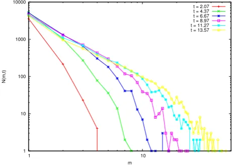
2.3.2 Time-Dependent Growth of Stationary Distributions

A trivial scaling for time-dependent growth of a stationary distribution can arise when

there is a constant injection of small masses into the system and a very large upper mass

size cutoff beyond which masses leave the system. That is, M→∞. This behaviour is

depicted Figure 2.3. Rescaling with respect to the evolution of the typical mass s(t) of

the system will recover the associated final stationary distribution. In this thesis we do not

attempt to apply inverse methods to transient evolutions of the mass distributions such as

these, although it is likely that the new methods developed in Chapter5could be applied.

1 10 100 1000 10000

1 10

N(m,t)

m

[image:32.595.200.432.402.566.2]

t = 2.07 t = 4.37 t = 6.67 t = 8.97 t = 11.27 t = 13.57

(33)

2.4 Non-stationary, Non-scaling Distributions

Lastly, we mention that for real clouds, rain formation is thought also to involve some

measure of fragmentation of droplets, as collisions at sufficient relative velocity cause some

break-up of the drops. In theory, depending upon the extent of fragmentation assumed for

a system theN(m,t) can eventually reach a steady state, as mass is recycled from larger

to smaller sizes. However, it is suggested that the durations required for steady states to

form are too long compared with real rain formation (except in the case of heavy rainfall)

[Prat and Barros,2007]. So it is possible that data from measurements of real clouds could

represent transient distributions.

A key question is whether these transient distributions exhibit scaling for some portion

of the mass distributions. If they do, then it might be possible to model at least part of

their behaviour using a kernel function of some degree of homogeneity. Otherwise inverse

(34)

Chapter 3

Monte Carlo Simulation

3.1 Monte Carlo Simulation of Cluster-Cluster Aggregation

In order to simulate the SCE, we made use of a method for the Monte Carlo (MC)

sim-ulation of chemical mixing introduced inGillespie [1976]. The full method in Gillespie

[1976] is designed to cope with coupled chemical reactions wherein a particular reaction

might have the form:

S₁+S₂−−−→R(1,2) 2S₃ (3.1)

Here, the subscripts indicate different chemical types: two different chemicals react to

provide two molecules of a third chemical at a rate governed by a function of the types,

R(1,2). For our simulations of cluster-cluster aggregation we are interested only in the

conservation of mass as clusters composed of the same material merge. So a cluster of

massiand a cluster of mass jaggregate to form a cluster of massi+jat a rate governed

(35)

Ai+Aj K(i,j)

−−−→Ai+j (3.2)

This simplified method is described inConnaughton et al.[2009] but we will repeat the

salient points here. The Monte Carlo process simulates the aggregation process (described

by the SCE) as a series of events. Each event is the aggregation of two masses. At time

t, the probabilityP(mˆ1,mˆ2,t) that an aggregation occurs between masses of two different

sizes, ˆm1and ˆm2, can be calculated according to:

P(mˆ₁,mˆ₂,t) = K(mˆ1,mˆ2)N(mˆ1,t)N(mˆ2,t) ∑∀m1,m2K(m1,m2)N(m1,t)N(m2,t)

(3.3)

WhereN(m,t)represents the number of clusters of massmpresent at timet. An event is

selected by forming the partial sums of theP(m1,m2,t)and then choosing one by matching

the partial sums to a uniform random number,r, generated on the interval[0,1). The event

indexed byi=n+1 is then selected by using,

n

∑

i=1

Pi(t)<r≤ n+1

∑

i=1

Pi(t) (3.4)

Equivalently, if we have the set of interaction typesS={(m₁,m₂):(m₁,m₂)∼(m₂,m₁)},

where(m₁,m₂)∼(m₂,m₁)denotes equivalence because of the symmetry of the kernel

func-tion, then the total number of types of possible aggregation events is given by NA =#S

(36)

Rtot(t) =

NA

∑

i=1

Ri(t) =

_∑

∀(m1,m2)∈S

K(m1,m2)N(m1,t)N(m2,t) (3.5)

The ordering of the sum over the pairs of mass sizes does not matter becauseris picked

randomly. Then for some index integern≤NA, it will be the case that,

n

∑

i=1

Ri(t)<Rtot(t)r≤

n+1

∑

i=1

Ri(t) (3.6)

Thus the event indexed byi=n+1 will be selected as the next aggregation event.

To modify this process to cope with the case of aggregation with a source of monomer

masses injected at rateJ, we simply count mass injection as another event type and form,

R_tot(t) =J+

NA

∑

i=1

Ri(t) (3.7)

The process of selecting which event type will occur next usingris similarly modified.

The total rate (at a particular time),Rtot(t), is used to parameterise the generation of an

amount of time that elapses in the system when an aggregation takes place. More

specifi-cally, the event interarrival waiting times are given by sampling from an exponential

distri-bution according to,

P(∆ˆt) =Re−R∆tˆ_,

(37)

This approach is valid because every aggregation event is considered to be an independent

event, of a type that would occur (if repeated in time) with a mean rate given by, for example,

K(m₁,m₂)multiplied by the time-dependent product of the mass densitiesN(m₁,t)N(m₂,t).

Hence, as the system evolves, what changes over time inRis the sum of the mean rates of

the Poisson distributed events as a function of changes in the productsN(m1,t)N(m2,t)for

each pair(m1,m2).

In the evolution of the SCE,N(m,t)is, strictly speaking, the mean-field average of the

number of clusters of sizemconsidered over all locations in a suitably large spatial domain.

However, physical particles moving through space do so at finite (diffusion or advection)

velocities, taking time to transit from one place to another, whereas the MC simulation (as

described above) is effectively zero-dimensional. Hence a tuning parameter must be added

to compensate for the absence of spatial movements by particles in order to make the mean

aggregation rates more realistic. The tuning parameter is in effect a suitable rescaling of

time. Given this tuning parameter,γ, the rates above are reformed as,

R_tot(t) =J+

NA

∑

i=1

γRi(t) =J+

∑

∀(m1,m2)∈S

γK(m1,m2)N(m1,t)N(m2,t) (3.9)

Then the (suitably tuned) MC simulation will approximate the mean-field in two main

ways. First, if a particular run of the simulator involves enough particles, then the Law

of Large Numbers suggests that aggregation events will occur at rates approximating their

mean rates. Secondly, an ensemble of runs can be averaged over to further improve the

(38)

3.2 Algorithmic Optimisations

In its raw form without optimisations, the Gillespie algorithm is not particularly fast,

because for each aggregation that occurs the recalculation of the event indexing is time

consuming. There are a number of ways to optimise the Gillespie algorithm, as reviewed

inMauch and Stalzer [2011]. Broadly speaking, they can be characterised according to

whether the number of chemical types remains fairly stable, or whether the number of

chemical types increases. For cluster-cluster aggregation, the increase in the number of

mass sizes over time is analogous to an expansion of the number of chemical types over

time, hence we will concentrate on this strand of algorithm development here. For the other

line of development, see its treatment inMauch and Stalzer[2011] and references therein,

and specific developments such asXiao and Ling[2007] andSlepoy et al.[2008]. The

sen-sitivity of cluster-cluster aggregation to the dynamics of the reaction rate propensities also

means that ‘tau-leaping’ method optimisations (see Gillespie [2007], Mauch and Stalzer

[2011] and references therein) are unlikely to be appropriate. (We will not consider

optimi-sations concerned only with parallelisation or GPU (graphics processing unit) utilisation,

as these are more concerned with the specifics of implementation.)

In general, when the Gillespie algorithm is running there are two main bottlenecks: The

first is the calculation to update the total event rate, and the second is finding which type

of reaction or aggregation event is the next one to take place. These processes are related.

For chemical systems with a limited number of reaction types it makes sense to have a

dependency graph between the reaction types, so that after a reaction has taken place and

the associated concentrations of chemical types have changed, only the minimum

num-ber of parts of the total reaction rate need to be updated. This dependency graph can be

implemented as a sparse matrix. For cluster-cluster aggregation the dependency graph is

(39)

[image:39.595.204.437.203.401.2]

(40)

are in place), and takes the form of a full square matrix. So while various optimisations

of the dependency graph are suggested inGibson and Bruck[2000],Cao et al.[2004], and

McCollum et al.[2006], they are not really relevant for cluster-cluster aggregation. Cao

et al.[2004], andMcCollum et al.[2006] also make use of the dependency graph to sort

reaction types in order of likelihood, but again, this is only useful for systems with a

re-stricted set of reaction types. Once the number of reaction types is allowed to expand in

potentially unlimited fashion, as in cluster-cluster aggregation, such sorting soon becomes

prohibitively expensive.

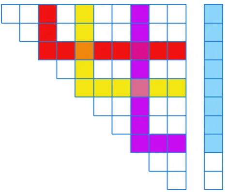
So the principal optimisation of interest for the Monte Carlo simulation of cluster-cluster

aggregation is the storage of partial sums for sections of the total event rate sum. This is

then combined with a binary search over the partial sums to obtain the reaction type index,

which considerably speeds up the process used in (3.6). For chemical systems this yields

an algorithm that runs inO(logNA)time [Li and Petzold,2006].

The use of partial sums also enables minimising the number of updates required for the

total event rate sum. There is an increase in the complexity of the code required to achieve

this, but (based on prototypes) we anticipate that the resulting algorithm should remain

O(M) in the worst case, whereM is the maximum mass size in the system. This should

permit Monte Carlo simulation of aggregation systems whereM∼108to run in reasonable

times. Figure3.1depicts how the reduction in the number of update operations is achieved.

3.3 Calibration of the Monte Carlo Simulation

3.3.1 Scaling Decay Case Distributions

(41)

particular problem. In the sub-gelation regime of the mean-field scaling decay case the

analytic solutions for both the time-dependent distributionN(m,t)evolutions and the

time-invariant rescaled distributionsΦ(z) of the constant kernel, Kc =1, and the sum kernel,

Ks(m1,m2) = (m1+m2)are known. Confining discussion to the scaling distributions, the

known scaling decay case solutions are, respectively [Leyvraz,2003]:

Φc(z) =4e−2z (3.10)

Φs(z) =

1

√

2πz3

e−2z _(3.11)

These are normalised distribution functions that presume that the initial mass of the

sys-temM1=1. Since, in the absence of gelation phenomena, the total mass of the system

remains constant, if the actual initial input,I0, of monomer massesm0=1 is some integer

amountI01 then in order to match the output from the Monte Carlo simulation and these

solutions, it is simply a case of dividing theN(m,t)data by the initial total massI0before

the rescaling is undertaken.

In order to match the outputs of the Monte Carlo simulation to the known time-dependent

analytic solutions forN(m,t)it is also necessary to take into account any scalar prefactor

in the kernel function that affects the rate of aggregation. So, for example, if we presume a

prefactor of1₄ in front of the constant kernel such that our simulation kernel isK=1₄, then

the rate of aggregation will be slowed by a factor of 4. Hence it should be the case that the

Monte Carlo timescale relates to the solution timescale according to1₄tMC=t.

If the behaviour of the Monte Carlo simulation accurately matches the known analytic

so-lutions for bothN(m,t)andΦ(z)outputs, then it can be presumed to be behaving properly.

(42)

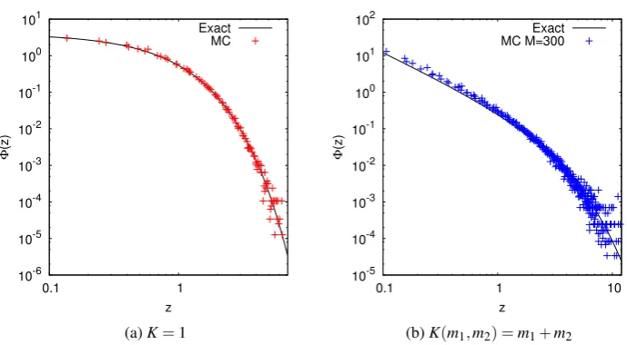
10-6 10-5 10-4 10-3 10-2 10-1 100 101

0.1 1

Φ

(z)

z Exact

MC

(a)K=1

10-5 10-4 10-3 10-2 10-1 100 101 102

0.1 1 10

Φ

(z)

z Exact MC M=300

[image:42.595.143.488.116.306.2]

(b)K(m1,m2) =m1+m2

Figure 3.2: Calibrations of the Monte Carlo simulation data from single runs withM=300 compared to the exact scaling solutions for (a) the constantK=1 kernel, and (b) the sum kernel. For the sum kernel, the discrepancy at smallzarises from finite system size.

in the limit of the Law of Large Numbers, eitherI0 has to be very large (relative to the

maximum mass size of the system), or more practically, a suitable batch of runs with

in-termediateI0 has to be performed and ensemble averaging of the results undertaken. We

found a number of runsnr=20 to be sufficient for the purposes of our research. However,

when finite system size can give rise to discrepancies from the large mass, large times

ex-act scaling solutionΦ(z)(as in Figure3.2b) comparisons of Monte Carlo data can also be

made against finite system size ODE integrations as a further check. We also undertook

these checks.

3.3.2 Stationary Distributions

For the case of stationary distributions N(m) calibration of the Monte Carlo results is

slightly more complicated, though the analytic solutions are known for arbitrary

(43)

Mbeyond which mass is discarded from the system. The key relationship in this case is

that for stable stationary distributions in the local regime, the rateJat which mass enters the

system matches the rate at which it leaves. For any given mass sizem, since∂tmN(m,t) =0

in the stationary state, the flux through that mass size is a constant that is independent ofm

[Connaughton et al.,2008]. Considering only the concentration of monomersN(m0) =N1

in the discrete case, withJ=1 under suitable normalisation, we have the relation:

1=

M

∑

m=1

K(m,1)NmN1 (3.12)

This represents a rescaled invariant flux relation. If we consider a mass injection at

rateJ>1, then if the kernel function remains unchanged, there has to be a corresponding

proportionate increase in the concentrations according to,

J=J

M

∑

m=1

K(m,1)NmN1=

M

∑

m=1

K(m,1)√JNm √

JN1 (3.13)

The relationship between the Monte Carlo simulation’s stationary distributionN_MC(m)

and the (stable) exact solutionN(m)is then given by:

N(m) = NMC√(m)

J (3.14)

However, this picture is further complicated if there is any additional prefactor added to

the kernel function to control the distribution evolution rates in the Monte Carlo simulation.

For example, if we add a prefactor of 1/Jto the kernel function, then the flux relation has

(44)

J=1 JJ

2

M

∑

m=1

K(m,1)NmN1= 1 J

M

∑

m=1

K(m,1)JNmJN1 (3.15)

In which case the relationship between the Monte Carlo simulation’s stationary

distribu-tionN_MC(m)and the corresponding (stable) exact solutionN(m)is modified to

N(m) = NMC(m)

J (3.16)

Hence the normalisation process has to take into account an interdependence between

kernel rates and mass concentrationsN(m)in the case of stationary distributions.

This exchange of weighting of factors between the kernel rates and the mass

concentra-tions also has consequences for the evolution of the system. Since the system is initially

devoid of mass, and mass is injected at rateJ, in the absence of any prefactor on the

ker-nel the total massM1 on the site is expected (deducing from (3.13)) to grow toward the

stationary state according to:

M1(t) =

M

∑

m=1 m

√

JN(m,t)∼Jt (3.17)

⇒ dM1

dt ∼

√

J (3.18)

In order to match up the timescales of the transient growth in both Monte Carlo

sim-ulation and an exact ODE integration of the SCE with J =1, it is desirable to map the

timescale of the Monte Carlo process so thatdtM1=1. Hence the timescale map becomes

(45)

Again, this process of remapping the timescales is complicated by the introduction of

a prefactor on the kernel of the Monte Carlo simulation. For the case given above with a

kernel prefactor of 1/J the equations for the transient growth become,

M1(t) =

M

∑

m=1

mJN(m,t)∼Jt (3.19)

⇒dM1

dt ∼1 (3.20)

Hence in this case there is no need to remap time to match up the solutions. The results

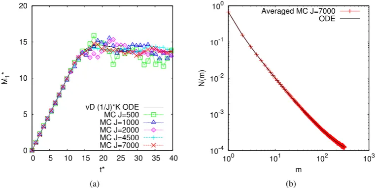
for this case are shown in Figure3.3.

0 5 10 15 20

0 5 10 15 20 25 30 35 40

M1

*

t*

vD (1/J)*K ODE MC J=500 MC J=1000 MC J=2000 MC J=4500 MC J=7000

(a)

10-4 10-3 10-2 10-1 100

100 101 102 103

N(m)

m

Averaged MC J=7000 ODE

[image:45.595.126.508.345.536.2]

(b)

(46)

In similar fashion, if the prefactor on the kernel is 1/√J then the adjusting factor for the

distribution concentrationsN(m,t)and the total massM1(t)isJ−

3

4, and the remapping of

time ist∗=t_MCJ14.

Summarising this in general formulae, we have,

J=γJβ

M

∑

m=1

K(1,m)NmN1 withγ=J−α ⇒β=α+1 (3.21)

N(m)∗=NMCJβ/2 (3.22)

t∗=t_MCJ1−β/2 _(3.23)

Lastly, for the stationary states, we found it was important to perform ODE integrations

of the SCE and match the data against our Monte Carlo simulation data, as once again finite

system size could affect the match to the exact analytic solutions by a scalar multiplying

factor. In Chapter5 we also provide a further stationary distribution generation method

using a Least Squares method, and this can be used for further checking of the Monte Carlo

simulation’s behaviour.

3.4 Collective Oscillations Around Stationary State Attractors

In the theory of wave kinetics it has been known for some time that only a subset of

kernel functions yield stable states with constant flux (in this case, of energy through the

wave spectrum) [Zakharov et al., 1992]. In aggregation kinetics, an equivalent notion is

that of kernels of the formK(m1,m2) =1₂(m₁µmν₂+mµ₂mν₁)that give rise to solutions in the

local regime, with |ν−µ|<1 [Connaughton et al., 2004]. For systems in the nonlocal

(47)

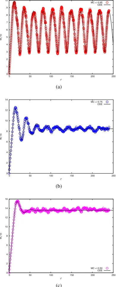
0 1 2 3 4 5 6 7 8 9 10

0 50 100 150 200 250

M1 *(t) t* MC +/-0.95 ODE (a) 0 2 4 6 8 10 12 14

0 50 100 150 200 250

M1 *(t) t* MC +/-0.75 ODE (b) 0 2 4 6 8 10 12 14 16

0 50 100 150 200 250

[image:47.595.221.417.116.599.2]

M1 *(t) t* MC +/-0.50 ODE (c)

(48)

state depending upon the upper cutoff mass size M. It was assumed that in real

aggre-gation systems, noise would typically disrupt concerted oscillations, allowing the system

to eventually approximate a stable state. So a thorough study of collective oscillations in

aggregation systems had not previously been undertaken.

During the course of the research for this thesis Monte Carlo simulations of finite systems

in the nonlocal regime, with kernel parameterisations that were known to yield unstable

dis-tributions with sizeable flux oscillations under exact ODE integration, were tested. Despite

the presence of significant noise throughout the system evolution, the Monte Carlo

simula-tions also exhibited sustained bulk flux oscillasimula-tions. Examples are shown in Figure3.4for

a system of sizeM=300 where the different effects obtained when the kernel is far away

from the local regime (Figure3.4a), on the border of the local regime (Figure3.4c), and at

parameterisation in between (Figure3.4b), can be seen. As a result of determining that the

oscillations remained in the presence of noise, further research on the topic of collective

oscillations (in the absence of noise) was then pursued inBall et al.[2012].

InBall et al.[2012] we investigated how the mass flux is carried from source to sink in

the nonlocal regime. It was found that for a range of values ofMthe numerical solution

retained persistent oscillations in the total mass on the site. This occurs even if the

simula-tion is started from an exact stasimula-tionary state and perturbed slightly. Analysis confirmed the

presence of a linear instability in the system, with the stationary state undergoing a Hopf

bifurcation to produce a limit cycle asMis increased.

The intuitive explanation of the mechanism that creates the oscillations is that the

nonlo-cality implies that larger masses aggregate with the smaller masses very efficiently. When

this occurs, the larger masses leave the system very rapidly, at the same time as the smaller

(49)

a delay before more of the larger masses are created, during which the remaining masses

in the spectrum aggregate more slowly. The smaller masses and the larger masses then

gradually replenish, with the creation of larger masses accelerating as more of the smallest

masses are injected into the system. The larger and smaller masses subsequently aggregate

strongly with each other, and cause another pulse of mass to exit the system rapidly.

From this explanation, it would be expected that the typical mass of the system, s(t)

would oscillate with a frequency matching that of the overall oscillations in the total mass

of the system. For the range of maximum massesM where oscillations occur, we might

also expect the amplitude of oscillations to grow asMis increased. From numerical

inves-tigations it was also seen that the rapid exit of larger masses almost reset the total mass in

the system to zero. In addition, it appeared that the mass in each pulse grew linearly in time

up to a maximum. However, the average mass flux through a particular mass size remained

constant.

From the above facts it was possible to deduce (seeBall et al.[2012]) that the typical

mass grows according to,

s(t)∼t2/(1−ν−µ) _(3.24)

Then estimating the period of oscillationτMas the time required for the typical mass to

reachMyields:

(50)

Assuming the linear growth of mass pulses in time according to Jt then provides the

amplitude of the oscillationsAMas:

AM∼JM(1−ν−µ)/2 (3.26)

Applying these equations to the data from (ODE) numerical simulations confirmed their

validity, providing evidence of the scaling of the oscillations in the total mass asM was

increased, for a fixed value of|ν−µ|[Ball et al.,2012]. For a fixed value ofM further

increase ofνrestores stability to the system for reasons that are not yet clear.

We remark that the kernel prefactorγ can be used to tune the Monte Carlo simulation,

controlling the aggregation rates of the system so that particular features can be better

ob-served. However, as was shown above in the discussion of the calibration of the Monte

Carlo system, the kernel prefactor has an effect on the total amount of mass found in the

system. The smallerγis, the more the aggregation rate is slowed, and (for some injection

J) the more mass will pile up on the site. The net effect is then that a smallerγ reduces

the amount of noise in the system, as the movement of single masses have proportionately

less effect on the total mass. The simulation then better approximates an ODE integration.

An ability to control the amount of noise in an evolution will be important for further

stud-ies of collective oscillations with noise and the phenomenon of quasicycles in aggregation

(51)

3.5 Noise-Driven Quasicycles Around Stationary State

Attrac-tors

For a system of finite mass spectrum containing a number of masses below a value

that would allow the Law of Large Numbers to reproduce ensemble averaging toward the

mean-field limit, the Monte Carlo process matches the Marcus-Lushnikov process (see

Al-dous[1999],Fournier and Giet[2004]). This makes Monte Carlo simulation an ideal tool

for investigating cluster-cluster aggregation phenomena in which noise plays a non-trivial

role. One such phenonemon is the capacity of intrinsic noise, caused by fluctuations in

population levels in a dynamical system, to generate and sustain noise-driven cycles (also

called stochastic cycles or quasicycles). These have been observed and discussed for some

time in connection with low-dimensional predator-prey-type models [Bartlett,1957] [

Nis-bet and Gurney,1976] [Nisbet and Gurney,1982] [Renshaw, 1991] [Gurney and Nisbet,

1998] [Mallick and Marcq,2003] [Morita et al.,2005] [McKane and Newman,2005] [

Mo-bilia et al.,2007]. Recently, mathematical techniques for the analysis of quasicycles have

reached maturity [Boland et al., 2008,2009] (see alsoShuda et al.[2009] and Tom´e and

de Oliveira[2009]) by exploiting an inverse system size expansion developed byvan

Kam-pen[2007].

Given the properties of collective oscillations investigated inBall et al.[2012] it is

per-haps not surprising that certain nonlocal parameterisations of aggregation systems of

par-ticular sizes should exhibit quasicycles in Monte Carlo simulation. In the following, we

present preliminary evidence that indicates that this is indeed the case.

Using the methods inBall et al.[2012] and some experimentation, we can construct an

ODE integration that represents a sensitive yet damped system, prone to oscillations of the

(52)

0 2 4 6 8 10

0 50 100 150 200 250 300 350 400 450

M1

*

t*

ODE vD (µ,ν) = +/-0.875, M=190 MC J=5000 MC J=10000

(a)

4.5 5 5.5 6 6.5

450 500 550 600 650 700 750 800 850

M1

*

t*

ODE vD (µ,ν) = +/-0.875, M=190 MC J=5000 MC J=10000

[image:52.595.198.435.108.486.2]

(b)

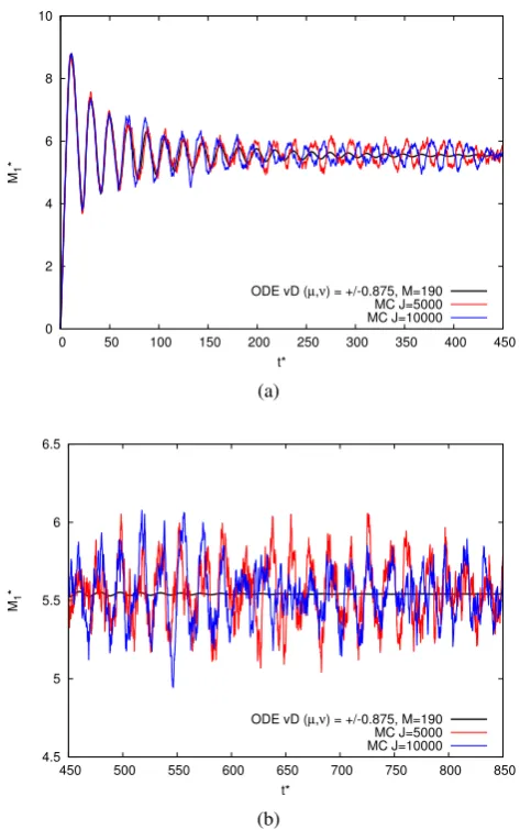
Figure 3.5: Comparisons of an ODE integration with Monte Carlo simulations withM= 190 for the “van Dongen” kernelKMC(m1,m2) =γ1₂(m₁µmν₂+mµ₂mν₁)withµ=0.875,ν=

−0.875, withJ_MC∈ {5000,10000}andγ=₂₅₀₀₀1 . Panel (a) shows times 0<t≤450; panel (b) zooms in on the interval 450<t≤850. The Monte Carlo data shown are for single runs without ensemble averaging.

though, the damping wins and the system will settle to a stable stationary distribution. By

feeding the same parameters into a Monte Carlo simulation of the aggregation system, and

controlling the amount of noise, it is possible to test whether the presence of noise will

(53)

In Figure3.5, we show the results for a system with upper cutoff massM=190 using

the kernelK(m₁,m₂) =1₂(m₁µmν

2+m

µ

2mν1) withµ =0.875,ν=−0.875. The system was

run for a period 0<t<860. In Figure3.5bit can be seen that the oscillations of the ODE

integration die away to zero, while the oscillations of correponding Monte Carlo simulations

with noisy evolution appear to be sustained. Most of the variance in the Monte Carlo time

series is caused by the noise (via the mechanism of stochastic amplification), so the real

question is whether the time series also contains evidence of a sustained sinusoidal signal.

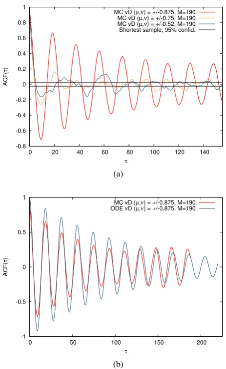
The theory in Ball et al. [2012] suggests that for systems of size M=190 but lesser

nonlocality, the damping effect should be stronger, and in the presence of noise long time

correlations in the total massM1(t)on the site should be lost. In Figure3.6awe compare

the (sample) autocorrelation functions (ACFs) ofM1(t)for the three kernels with(µ,ν)∈

{±0.875,±0.75,±0.52}. Only the(µ,ν) =±0.875 case exhibits sinusoidal correlations

over large lag timesτ. In the other two cases noise acts disruptively.

Moreover, by comparing the ACFs of the Monte Carlo and ODE integrations for the

(µ,ν) =±0.875 case, we see in Figure3.6bthat at large lag timesτ the ACF of the Monte

Carlo integration has a fixed amplitude and frequency, while that of the ODE integration

continues to decay. This suggests that noise is having a driving effect sustaining the

under-lying sinusoidal signal in the time series in the manner of a phase-remembering quasicycle

[Nisbet and Gurney,1982] [Renshaw,1991].

It is suggested in Boland et al. [2008, 2009] that generalisations of the mathematical

methods therein could be deployed against high dimensional systems. (C.f. van Dongen

[1987b] where fluctuations ofN(m,t)in decay case evolutions are studied using the inverse

system size expansion.) However, the specifics of adapting the analysis to stationary state

Determining cluster cluster aggregation rate kernals using inverse methods

University of Warwick institutional repository: http://go.warwick.ac.uk/wrap

A Thesis Submitted for the Degree of PhD at the University of Warwick

http://go.warwick.ac.uk/wrap/57480

This thesis is made available online and is protected by original copyright.

Please scroll down to view the document itself.

Determining Cluster-Cluster Aggregation

Rate Kernels Using Inverse Methods

Peter P. Jones

Contents

List of Figures

List of Tables

Acknowledgments

Declarations

Abstract

Chapter 1

Introduction

1.1

Prelude

1.2

The Contemporary Relevance of the Inverse Problem

1.3

Thesis Structure

1.4

A Note on Terminology

Chapter 2

Cluster-Cluster Aggregation and the

Smoluchowski Coagulation Equation

2.1

General Properties

∑

∑

∑

∑

∑

2.2

Decay Case Distributions

2.3

Stationary Distributions

2.4

Non-stationary, Non-scaling Distributions

Chapter 3

Monte Carlo Simulation

3.1

Monte Carlo Simulation of Cluster-Cluster Aggregation

∑

∑

∑

∑

∑

∑

∑

∑

∑

3.2

Algorithmic Optimisations

3.3

Calibration of the Monte Carlo Simulation

∑

∑

∑

∑

∑

∑

∑

∑

3.4

Collective Oscillations Around Stationary State Attractors

3.5

Noise-Driven Quasicycles Around Stationary State

Attrac-tors

_∑