Abstract — This paper compares the performance of Mel-Frequency Cepstral Coefficients (MFCCs), their deltas and delta-deltas, which are conventionally used in the forensic voice comparison arena, to an alternative set of features, namely the Complex Cepstral Coefficients (CCCs). The performance of CCCs has been found to outperform MFCCs in terms of the accuracy and precision of the likelihood ratio results. It is hypothesized that this is because CCCs intrinsically carry more speaker-specific information than MFCCs, this being specifically related to the glottal shaping and lips radiation filters of the speech production model.
Index Terms — cepstral coefficients, forensic voice comparison, likelihood ratio.
I. INTRODUCTION
NALYSIS of speech recordings can play a crucial part in determining the identity of an offender in a court of law. The speech samples are normally compared on the basis of various discriminative parameters, such as formants, formant trajectories and Mel-frequency cepstral coefficients (MFCCs). This study investigates the comparative performance of MFCCs with an alternative set of cepstral coefficients, specifically the complex cepstral coefficients (CCCs).
MFCCs, including their first and second derivative parameters (i.e., deltas and delta-deltas), have been used in speech forensics for a while and have been shown to produce good results [1]-[4]. MFCCs are broadly a perceptual based feature set. CCCs, on the other hand, tease out information relating to the speech production process [5]. Currently CCCs are not used in the speech forensics arena. This is likely related in part to the potential sensitivity of this feature set to transmission artifacts such as channel noise, channel phase distortion, etc. However, speech
Manuscript received July 7, 2014; revised July 30, 2014.
B. B. T. Nair is a PhD student at the Dept. of Electrical and Computer Engineering, Faculty of Engineering, The University of Auckland (e-mail: [email protected]).
E. A. Alzqhoul is a PhD student at the Dept. of Electrical and Computer Engineering, Faculty of Engineering, The University of Auckland (e-mail: [email protected]).
B. J. Guillemin is a Senior Lecturer at the Dept. of Electrical & Computer Engineering, Faculty of Engineering, The University of Auckland (phone: (09) 373 7599 Ext. 88190, Fax: (09) 373 7461, e-mail: [email protected]).
transmitted across a mobile phone network does not get directly impacted by such factors, but rather in a highly indirect manner [6]. Given that mobile phone speech is being increasingly used as evidence in courts of law, we have decided to take a fresh look at this feature set and compare its performance in FVC to more commonly used feature sets. Though the comparison process in this paper has been performed using studio quality recordings, which does not reflect a realistic forensic scenario, we believe the analysis results presented nonetheless provide an indication of the speaker-specific information contained in each feature set.
The following four experiments are based on the analysis of vowel segments (specifically, one monophthong and two diphthongs). Different realizations of the MFCCs parameters have been considered. With the first experiment, MFCCs have been extracted from the entire vowel segment. The second and third experiments use MFCCs, but they incorporate deltas and delta-deltas, respectively, these being extracted by segmenting the speech into stationary frames of 30ms. The fourth experiment uses CCCs that have been again extracted from the entire vowel segment.
The likelihood-ratio framework has been used in our experiments to quantify the strength of speech evidence. Among the different probabilistic models available, such as Multivariate Kernel Density (MVKD) [7], Gaussian Mixture Model-Universal Background Model (GMM-UBM) [8] and Principal Component Analysis Kernel Likelihood Ratio (PCAKLR) [9], the latter approach has been chosen for this investigation because of its ability to handle large number of parameters, such as is the case with cepstral coefficients, without any computational issues. It also has been found to provide comparable results to the MVKD analysis when used with a small number of parameters [9]. The performance of MFCCs and CCCs in FVC has been analysed by comparing their corresponding accuracy and precision. The results are shown using Tippett plots and the performance measuring tools include log-likelihood-ratio cost
(
C
llr)
, Average Probability Error Plots (APE) and Credible Interval.The remainder of this paper is structured as follows. Details of CCCs and MFCCs are discussed in the following section. This is followed by a brief overview of PCAKLR along with a description of the performance measuring tools
Comparison between Mel-Frequency and
Complex Cepstral Coefficients for Forensic
Voice Comparison using a Likelihood Ratio
Framework
Balamurali B. T. Nair, Esam A. S. Alzqhoul, Bernard J. Guillemin
used in this investigation. Section III discusses the experimental methodology, followed in Section IV with the discriminative performance of the aforementioned speech parameters in FVC. Discussions and conclusions appear in Section V.
II. BACKGROUND INFORMATION
A. Cepstral analysis
When applied to speech, cepstral analysis (often referred as homomorphic filtering [10]) can be used to separate out the various aspects of speech production process. Cepstral analysis is defined as the inverse Fourier transform of the logarithm of the Fast Fourier Transform (FFT) of the signal [5]. A number of different sets of cepstral coefficients exist. The term cepstrum typically refers to the set obtained when the logarithm function is applied to the magnitude of the FFT components only. When it is applied to both the magnitude and phase component of speech the resulting set is referred to as the complex cepstrum. Fourier analysis of the speech signal is used to convert the convolution between the source and filter components in the time domain into a product of their corresponding representations in the frequency domain. The logarithm operator transforms this product operation into a sum of both components. The inverse Fourier transform is then used to bring the separated components back into the time domain (quefrency domain) [5], [11]. The resultant cepstral coefficients characterize the slow and fast varying components of speech. Slow varying components (e.g. pitch) get concentrated in the upper part of the cepstral domain, whereas the fast varying components (e.g. the vocal tract filter) get concentrated in the lower part.
Complex Cepstral Coefficients
When the complex cepstrum analysis is applied to speech, the components of the speech production model will be separated as described in (1) - (5) [5].
* .
*
*
s n
p n
A g n
v n
r n
(1)
( )
.
S z P z A G z V z R z (2)
( )S z P z H z (3)
{log } log log
IFFT S z IFFT P z H z (4)
( )
ˆ
( )
ˆ )
(
ˆ
s n
p n
h n
(5)where * is the convolution operator, s is the speech signal,
p is the excitation signal (assumed impulse like signal for voiced speech), g is the glottal shaping filter with gain A, v is the vocal tract filter, r is the lips radiation filter and H(z) is the overall filter response in the frequency domain. The glottal shaping filter, G(z), is typically a stable, anti-causal filter with poles located at the origin and zeroes outside the unit circle. The vocal tract filter, V(z), is typically an all pole filter with all of its poles inside the unit circle. The lip radiation filter, R(z), typically has a pole at the origin and a zero inside the unit circle [5].
Applying the complex logarithm to S(z) and then inverse Fourier transforming produces a set of complex cepstral coefficient (as in (4) and (5)),
s n
ˆ( ).
This is the summationof two subsets of coefficients,
h n
ˆ( )
(arising from H(z)) andˆ( )
p n
(arising from P(z)).h n
ˆ( )
will comprise of both causal and anti-causal components, the causal components arising from V(z) and R(z), and the anti-causal components arising from the zeroes of G(z).p n
ˆ( )
will also comprise of causal and anti-causal components.h n
ˆ( )
dominates the lower part ofs n
ˆ( ),
whereasp n
ˆ( )
dominates the upper part.Mel Frequency Cepstral Coefficients
MFCC analysis focuses on the perceptually relevant aspects of the speech spectrum. The speech signal is converted to the frequency domain using the Discrete Fourier Transform (DFT). The next step is estimating how much energy exists in various regions of the frequency domain. This is motivated by the fact that the human ear responds linearly at different frequencies. This non-linear response to frequencies is best represented by the Mel-scale shown in (6):
( ) 1125 ln 1
700
f
M f
(6)where f is the frequency and M(f) is the equivalent Mel-scale frequency. The energy is then estimated over a set of overlapped Mel-filter banks by computing the power spectrum of the speech signal and then summing up the energies in each filter bank region. Once the filter bank energies are computed, the logarithm operator is applied. Unlike CCCs, which use IFFT in their last step, the MFCC extraction performs the Discrete Cosine Transform (DCT) on the logarithm of the energies computed. The resultant set,
MFCC(n), as given in (7), is causal,
1
1 2 1
log cos
2 R
r
MFCC n MF r r n
R R
(7)where, MFCC(n) is the nth MFCC coefficient extracted from a particular speech segment using R triangular filters and MF(r) is the mel-spectrum for the rth filter [5]. It is a common practice to use deltas and delta-deltas along with MFCCs to capture the dynamic aspects of the speech signal [1]. These are simply the first and second order derivatives of MFCCs over a range of short-term speech frames.
Given that CCCs arise from taking the complex logarithm of the FFT of s(n) (both magnitude and phase), whereas MFCC arise from taking the logarithm of the magnitude of FFT only, the set of CCCs should potentially contain more speaker-specific information than MFCCs, and thus the motivation for this study.
B. Likelihood ratio (LR) framework
( | )
( | )
p
d
p E H LR
p E H
(8)
where
p E H
( |
p d,)
is the conditional probability of the evidence given the prosecution and defence hypothesis, respectively. LR values significantly greater than one support the prosecution hypothesis and values significantly less than one support the defence hypothesis. Being an easier metric to analyze, log likelihood ratios (LLRs) are often calculated from LRs. Like LR, the magnitude of the LLR is a measure of the strength of evidence, but its sign indicates whether this is in favor of prosecution or defence. Positive values favour the former, while negative values favour the latter.For the following set of experiments, PCAKLR has been chosen for computing LRs [9]. In PCAKLR, firstly the speech parameters are transformed into a new set of uncorrelated parameters using principal component analysis. Secondly, a LR value for each of these transformed parameters is determined using univariate kernel density analysis (UKD). Given the assumption of uncorrelated parameters, the individual LRs are multiplied to produce a final LR value. In UKD, the LR is calculated using the following equation [15].
2 2
2 2 2
2 2
2 2
2 2 2 2 2 2
2( ( )( ))
2
1
2( ) 2( )
1 1
i k
i i
k k
m n w z x y
k m n s
a
i
m x z n y z
m s n s
k k i i
Ke
e
LR
e
e
(9) where, 2 2 k 2 i k i 1(z
z)
s
1
ˆσ
k
k
(10)
2 k N j 2 2i 1 j 1
z z
1
σ
σ
k 1
N 1
(11) 2 k N j 2i 1 j 1
(z z )
1
σ
k
N
ˆ
1
(12)
2 2 2 2 2 2
k k
2 2 2
k
k σ
m s λ . σ
n(s λ )
K
aσ mn. σ
(m n)(s λ )
(13)x
y
1
1
;
;
mx
ny
z
a
w
2
m
n
m n
(14)x, y
are the means of offender and suspect data respectively.z
jis the mean of an individual speaker data in the background.
2,
s
k are the within and between speaker variances respectively.σ
2 is the combined suspect and offender variance.λ
is a smoothing factor. N, k are the number of tokens per speaker and the number of speakers in the background respectively. Finally, m and n are the number of tokens of the offender and suspect data respectively.C. Log-Likelihood ratio cost
The accuracy of a FVC experiment measures the closeness of the obtained result to its true value. Log-likelihood ratio cost (
C
llr ) is one such tool recommended in the speech forensics arena [16]-[18], defined as
so do
j i
N N
2 2 do
i 1 j 1
so so do
1 1 1 1
log 1 log 1 LR
2 N LR N
llr C
(15) so doN , N
are the number of same- and different-speaker comparisons andLR
so,
LR
do are their corresponding LRs. The lower theC
llr value, the more accurate is the analysis and vice versa.D. Credible interval (CI) as a precision measure
The precision of a FVC analysis is the amount of variation expected in the LR due to the variability in the source. Once CI is calculated, one can be confident that the true LR value lies within the 95% of it. Of the two approaches proposed for calculating CI, the non-parametric approach is the one typically used [19], [20] and this has been chosen for the following experiments to measure precision.
E. Tippett plot
A Tippett plot is a graphical way of presenting the LLR results of a FVC analysis. It represents the cumulative proportion of LLR results obtained for the same- and different-speaker comparisons [12], [21]. As a large positive LLR value supports the prosecution and a larger negative value the defence, the further apart are the same-speaker (to the right) and different-speaker curves (to the left), the better are the results.
F. Applied Probability of Error (APE) plot
The losses in the
C
llr value can be teased out using an APE plot [22], [23]. Two major losses: discrimination (C
llr min) and calibration loss (C
llr cal) are present in every FVC system. The former corresponds to the lowestC
llr that can be achieved while preserving the discrimination power, while the latter is the difference between the obtainedllr
C
value andC
llr min. An APE plot comprises a number of APE curves and bar graphs.APE curves plot the error rate against the logit prior and they include three curves: dashed, solid and dotted with circular marker. The dashed curve shows error rate of the optimized LLRs, whereas the solid curve shows the error rate of the system under evaluation. Finally, the dotted curve with circular marker shows the error rate of the reference system (
C
llr0
). The bar graph gives the area under the dashed and solid curves. Importantly, the height of the bottom bar givesC
llr minand is proportional to the area under the dashed curve, while the height of the top bar givesllr cal
III. METHODOLOGY A. Speech database and Speech parameters
The XM2VTS database has been used in our experiments. It includes speech recordings of 295 speakers [24]. Speakers were recorded on four different occasions separated by one month and during each session every speaker read three sentences twice. Only male speakers have been considered for our experiments. Among the 156 males, 26 were discarded as they either sound less audible or appeared to have a different accent from the rest. The vowel segments /aI/, /eI/ and /i/ were extracted from the words “nine”, “eight” and “three”, respectively, from the first two sentences for every speaker.
The database with 130 speakers has been divided into three groups: 44 speakers for the Background set, 43 speakers for the Development set and 43 speakers for the Testing set. Note that the sole purpose of the Development set is to train the logistic regression fusion system [25], the resultant weights of which are used to combine LRs calculated from individual vowels.
In summary, four tokens of three different vowels (two diphthongs and one monophthong) from three non-contemporaneous recordings were used in the following experiments. Using three different sessions, two same-speaker comparisons and three different-speaker comparisons are possible.
C
llr values were calculated from the mean LR values and will be referred to as MeanC
llr.
Credible interval was calculated by finding the variation in LR values over a set of speech recordings for a particular comparison.B. Experimental methodology
A number of experiments have been considered. In Experiment 1, a set of MFCCs extracted from the entire vowel segment have been used. Experiment 2 uses both MFCCs as well as deltas. With this experiment, a vowel segment has been segmented into 30ms Hamming windowed frames. MFCCs have then been computed for each and the average of these has produced a set of Mel-frequency cepstral coefficients. Deltas are computed by determining difference of MFCCs in adjacent frames. Exactly the same procedure has been used in Experiment 3 which includes MFCCs, deltas and delta-deltas. With Experiment 4, CCCs have been calculated from the entire speech segment.
In the first Experiment, 23 MFCCs were extracted from the entire vowel segment (Note: all the DCT coefficients have been considered here). The maximum number of MFCCs that can be extracted is determined by the data’s sampling frequency [5]. In our experiments we have down-sampled the speech data to 8 kHz, this being the standard value used in both the landline and mobile phone arena. At 8 kHz sampling frequency a maximum of around 23 MFCCs can be extracted. We felt it important in this investigation to use as many parameters as possible in a feature set in order to ensure fairness when comparing results between feature sets. Experiments 2 and 3 follow the conventional way of MFCC extraction by segmenting a speech segment into frames of 30 ms. MFCCs along with their corresponding
deltas and delta-deltas, extracted from short-term speech segments, have been used around for a while and have shown good results in respect to FVC analysis. For Experiment 2, 12 MFCCs and 12 deltas were considered. An additional 12 delta-deltas have been added in Experiment 3. A maximum of 12 MFCCs are traditionally used when undertaking an analysis on a frame-by-frame basis because of the small amount of data that is then being analysed, which introduces noise into the higher-order MFCC filter banks. For Experiment 4, a total of 100 CCCs were considered (50 Causal and 50 anti-causal components). This number has been chosen based upon early research examining the use of CCCs when applied to speech [5]. Again, we wanted to use the maximum number of parameters per feature set that it made sense to use. The performance of FVC using these parameters was analyzed using
C
llr and CI.IV. EXPERIMENTAL RESULTS
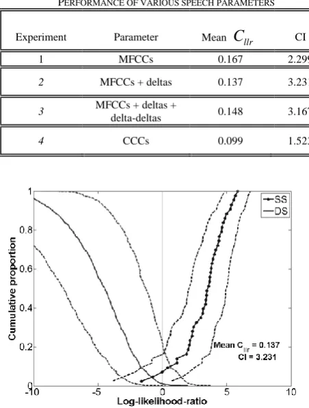
Table 1 compares the resulting FVC performance for each of the experiments described. On the basis of both
C
llr and CI, it is clear that CCCs (i.e., Experiment 4) have outperformed the other experiments. The combination of MFCCs and deltas (i.e., Experiment 2) has resulted in a marginally better performance in terms of accuracy among the various MFCC realizations. However, its precision seems significantly worse. MFCCs tend to have larger variation when computed over a range of stationary speech frames. In contrast, those extracted from the entire speech segment reflect less variation and result in a better precision.TABLEI
PERFORMANCE OF VARIOUS SPEECH PARAMETERS
Experiment Parameter Mean
C
llr CI1 MFCCs 0.167 2.299
2 MFCCs + deltas 0.137 3.231
3 MFCCs + deltas +
delta-deltas 0.148 3.167
4 CCCs 0.099 1.523
[image:4.595.305.531.462.760.2]The results have been further analyzed using Tippett plots. Fig. 1 shows a Tippett plot for the best performing MFCC set in terms of accuracy (i.e., Experiment 2). Tippett plots of the other MFCC-based sets are very similar to those of Fig. 1 and have not been shown. Fig. 2 shows the corresponding Tippett plot for CCCs (i.e., Experiment 4). In the Tippett plots shown, the solid curve with dotted marker rising towards the right represents the same-speaker comparison results and the solid curve rising towards the left the different-speaker comparison results. The dashed lines on either side of the same- and different-speaker results curves represent the variation found in a particular LLR.
Fig. 2. Tippett plot showing FVC performance using CCCs.
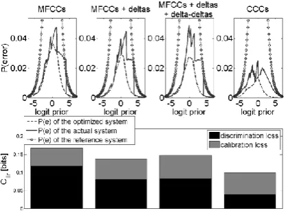
Fig. 3. APE plots showing the losses in Cllr for various speech feature sets.
It might be concluded from Fig. 1 and 2 that MFCCs have outperformed CCCs (in Fig. 1 the curves are further apart than they are in Fig. 2). However, the performance of an FVC experiment in the vicinity of the LLR = 0 decision boundary is more important than the performance of higher magnitude LLRs. As can be seen from Fig. 1 and 2, CCCs have outperformed MFCCs in this region for the same-speaker comparisons. However, MFCCs have outperformed CCCs in terms of different-speaker comparisons. The proportion of same-speaker misclassifications is lower for CCCs (almost none) compared to MFCCs, but the opposite is true for different-speaker misclassifications. For larger LLR magnitudes, MFCCs have outperformed CCCs for both same- and different-speaker comparisons. The APE-plot in Fig. 3 shows that the improvement in
C
llr when using CCCs is attributable to the improved discriminationperformance of this feature set (i.e., CCCs have resulted in a llr min
C
of 0.040 as compared to MFCCs’ 0.117, MFCCs + deltas’ 0.082 and MFCCs + deltas + delta-deltas’ 0.083). However, the calibration performance(
C
llr cal)
for all these feature sets is comparable (i.e., CCCs have resulted in allrcal
C
of 0.059 as compared to MFCCs’ 0.050, MFCCs + deltas’ 0.055 and MFCCs + deltas + delta-deltas’ 0.065).V. CONCLUSIONS
This paper has compared the performance of MFCCs with CCCs in the context of FVC. The result is shown for clean speech. It is clear from the results that CCCs have outperformed MFCCs. This is specifically in terms of discrimination. The results presented suggest that CCCs fundamentally contain more speaker-specific information. This is of potential interest when analyzing mobile phone speech because the speech in that arena is never directly impacted by transmission artifacts such as channel noise and channel distortion. However, the extent to which CCCs are impacted by other factors in a real forensic situation, such as mismatch in recording conditions between suspect and offender data, still needs to be investigated.
REFERENCES
[1] S. Furui, "Speaker-independent isolated word recognition using dynamic features of speech spectrum," IEEE Transactions on Acoustics, Speech and Signal Processing, vol. 34, pp. 52-59, 1986. [2] E. Enzinger, C. Zhang, and G. S. Morrison, "Voice source features
for forensic voice comparison–an evaluation of the GLOTTEX R G software package," 2012.
[3] D. Vandyke, P. Rose, and M. Wagner, "The voice source in forensicvoice-comparison: a likelihood-ratio based investigation with the challenging yafm database," Proceedings International Association of Forensic Phonentics and Acoustics, 2013.
[4] C. C. Huang, J. Epps, and C. Zhang, "An Investigation of Automatic Phonetic-Unit Selection for Forensic Voice Comparison," SST 2012, Sydney, Australia, 2012.
[5] L. R. Rabiner and R. W. Schafer, Theory and application of digital speech processing: Pearson, 2009.
[6] E. A. Alzqhoul, B. B. Nair, and B. J. Guillemin, "Speech Handling Mechanisms of Mobile Phone Networks and Their Potential Impact on Forensic Voice Analysis," SST 2012, Sydney, Australia, 2012. [7] C. G. Aitken and D. Lucy, "Evaluation of trace evidence in the form
of multivariate data," Journal of the Royal Statistical Society: Series C (Applied Statistics), vol. 53, pp. 109-122, 2004.
[8] D. A. Reynolds, T. F. Quatieri, and R. B. Dunn, "Speaker verification using adapted Gaussian mixture models," Digital signal processing, vol. 10, pp. 19-41, 2000.
[9] B. B. Nair, E. A. Alzqhoul, and B. J. Guillemin, " Determination of Likelihood Ratios for Forensic Voice Comparison Using Principal Component Analysis," International Journal of Speech Language and the Law, vol. 21(1), pp 83-112, 2014.
[10] A. Oppenheim and R. Schafer, "Homomorphic analysis of speech," IEEE Transactions on Audio and Electro acoustics, vol. 16, pp. 221-226, 1968.
[11] B. P. Bogert, M. J. Healy, and J. W. Tukey, "The quefrency alanysis of time series for echoes: Cepstrum, pseudo-autocovariance, cross-cepstrum and saphe cracking," in Proceedings of the symposium on time series analysis, 1963, pp. 209-243.
[12] G. S. Morrison, "Forensic voice comparison," Expert Evidence, vol. 40, pp. 1-105, 2010.
[13] P. Rose, Forensic speaker identification: CRC Press, 2004.
[14] J. Gonzalez-Rodriguez and D. Ramos, "Forensic automatic speaker classification in the “Coming Paradigm Shift”," in Speaker Classification I, ed: Springer, 2007, pp. 205-217.
[image:5.595.61.271.400.555.2][16] G. S. Morrison, "Measuring the validity and reliability of forensic likelihood-ratio systems," Science & Justice, vol. 51, pp. 91-98, 2011.
[17] G. S. Morrison, "Forensic voice comparison and the paradigm shift," Science & Justice, vol. 49, pp. 298-308, 2009.
[18] J. Gonzalez-Rodriguez, P. Rose, D. Ramos, D. T. Toledano, and J. Ortega-Garcia, "Emulating DNA: Rigorous quantification of evidential weight in transparent and testable forensic speaker recognition," IEEE Transactions on Audio, Speech, and Language Processing, vol. 15, pp. 2104-2115, 2007.
[19] G. S. Morrison, T. Thiruvaran, and J. Epps, "Estimating the precision of the likelihood-ratio output of a forensic-voice-comparison system," in Proceedings of Odyssey, 2010, pp. 63-70.
[20] G. S. Morrison, C. Zhang, and P. Rose, "An empirical estimate of the precision of likelihood ratios from a forensic-voice-comparison system," Forensic science international, vol. 208, pp. 59-65, 2011. [21] D. Meuwly and A. Drygajlo, "Forensic speaker recognition based on
a Bayesian framework and Gaussian Mixture Modelling (GMM)," in 2001: A Speaker Odyssey-The Speaker Recognition Workshop, 2001. [22] N. Brummer, L. Burget, J. H. Cernocky, O. Glembek, F. Grezl, M. Karafiát, D. A. van Leeuwen, P. Matejka, P. Schwarz, and A. Strasheim, "Fusion of heterogeneous speaker recognition systems in the STBU submission for the NIST speaker recognition evaluation 2006," IEEE Transactions on Audio, Speech, and Language Processing, vol. 15, pp. 2072-2084, 2007.
[23] N. Brümmer and J. du Preez, "Application-independent evaluation of speaker detection," Computer Speech & Language, vol. 20, pp. 230-275, 2006.
[24] K. Messer, J. Matas, J. Kittler, J. Luettin, and G. Maitre, "XM2VTSDB: The extended M2VTS database," in Second international conference on audio and video-based biometric person authentication, 1999, pp. 965-966.