Voltage Control in Smart Grids: An Approach
Based on Sensitivity Theory
Morris Brenna1, Ettore De Berardinis2, Federica Foiadelli1, Gianluca Sapienza3, Dario Zaninelli1
1Politecnico di Milano – Department of Energy, Milan, Italy; 2
CESI S.p.A., Milan, Italy; 3Politecnico di Milano – Department of Energy in Collaboration with ENEL Distribuzione S.p.A., Milan, Italy.
Email: [email protected]
Received March 30th, 2010; revised May 25th, 2010; accepted May 31st, 2010
ABSTRACT
Due to the development of Distributed Generation (DG), which is installed in Medium-Voltage Distribution Networks (MVDNs) such as generators based on renewable energy (e.g., wind energy or solar energy), voltage control is currently a very important issue. The voltage is now regulated at the MV busbars acting on the On-Load Tap Changer of the HV/MV transformer. This method does not guarantee the correct voltage value in the network nodes when the distributed generators deliver their power. In this paper an approach based on Sensitivity Theory is shown, in order to control the node voltages regulating the reactive power exchanged between the network and the dispersed generators. The automatic distributed voltage regulation is a particular topic of the Smart Grids.
Keywords: Voltage Regulation, Reactive Power Injection, Distributed Generation, Smart Grids, Sensitivity Theory, Renewable Energy
1. Introduction
Due to the development of Distributed Generation (DG), which is installed in Medium-Voltage Distribution Net- works (MVDNs) such as generators based on renewable energy (e.g., wind energy or solar energy), voltage con- trol is currently a very important issue.
The voltage of MVDNs is now regulated acting only on the On-Load Tap Changer (OLTC) of the HV/MV tra- nsformer [1]. The OLTC control is typically based on the compound technique, and this method does not guarantee the correct voltage value in the network nodes when the generators deliver their power [2,3].
When a generator injects power in the network, the vo- ltage tends to rise. In HV networks this phenomenon ha- ppens mainly when reactive power is injected, because the resistance is negligible if compared with the induc-tive reactance [4]. Instead in MVDNs the resistance is not negligible and the result is that an injection of active power also increases the voltage.
In other words the so-called Pθ - QV decoupling [5], which is a typical of HV networks, is inexistent in MVDNs. The P variations are “coupled” with the voltage variations.
If no precautions are taken, in particular network con- ditions the overcome of the maximum admissible voltage can happen in any nodes.
When a generator injects power, the voltage rises in all network nodes, but some nodes are mainly influenced than others by the power injection. This influence can be obtained using a Sensitivity method.
In this paper an approach based on Sensitivity The- ory is shown, in order to control the network voltage us- ing the reactive power exchanged between network and the distributed generators. This approach allows to con-trol the voltage in the long term period. Besides, fast- dynamic voltage disturbances are not taken into account [6].
After the theoretical analysis, a numerical example is shown, in order to validate the proposed theory.
The proposed method differs from the others used in HV networks analysis, based on the Jacobian Matrix [1,2-4] and its application is easy.
The topological proprieties that results from the th- eoretical analysis imply that the proposed sensitivity me- thod can be easily implemented in automatic voltage control devices, in order to obtain the distributed voltage regulation.
The automatic voltage regulation in a distributed man- ner is a typical topic of the Smart Grids context.
studied, referring to a MV test network, composed by four nodes. Finally, in Section 4, a numerical application is presented, in order to validate the proposed theory.
2. The Proposed Criteria to Control the
Network Voltage with Distributed
Generation
Many methods can be used to control the voltage in ne- twork nodes (network voltages). The proposed method varies the reactive power exchanged between the gen-erators and the network while maintaining the OL-TC in a fixed position for a particular load condition.
Let us suppose that the Automatic Voltage Regulator (AVR) that controls the OLTC maintains the MV bus-bar voltage at the rated value (1 p.u.), assuming that the transformer taps are adequate.
For passive grids, when no generators are connected to the MVDN, the voltage profile (VP; i.e., the voltage values along a line) decreases monotonically (see profile a in Figure 1) due to the load absorptions. When the gen- erators are connected and inject power into the MVDN, the nodal voltages increase and the VP is no longer monotonic, as shown in profile b in Figure 1 (profile b). This phenomenon also occurs if generators work at unitary power factor (i.e., only active power is injected due to the non-negligible network resistance) [7].
It is important to note that, in steady-state, the con- dition maintained at the MV busbar by the AVR decouples the MV feeders, and the result is that each feeder works without the influence of the other lines. In other words, the loads and generators connected to other feeders do not influence the VP of the considered line.
Typically, the generators installed in Smart Grids are based on renewable energy; therefore, their power-time profiles are unknown. Due to the high generated power and a possibly low load condition, the voltage in some nodes can thus exceed the maximum admissible value (Vmax; i.e., the voltage threshold [8]) defined by the
standards.
Of course the voltage threshold is strictly related with the settings of the voltage relays installed in the network, e.g. at the generator nodes [9].
~
G G
x
V
n
V b a
Load
, B ref
V AVR VB Generator MV feeder MV busbar
/
[image:2.595.308.536.604.702.2]HV MV
Figure 1. Voltage profiles in a MV feeder with and without Distributed Generators
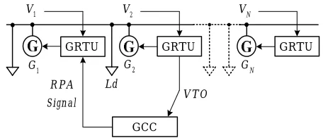
If the generators are able to control the injected or absorbed reactive power, the network voltage profiles can be modified by acting on the reactive powers. It is clear that each controllable generator needs a Generator Remote Terminal Unit (GRTU) that is connected to a central control system to set the generator reactive power, (i.e., to control the exciter of the synchronous generators [1] or act on the inverter control if the generator is in-verter-based) [10,11]. In this work, the central control is called the Generator Control Centre (GCC). In addition, we use a hierarchical control structure [12,13].
Let us suppose that the voltage is measured only in the generator nodes by the GRTUs. This assumption does not affect the generality of the proposed method because a Measuring Remote Terminal Unit connected to the GCC can be installed in each node that must be controlled.
When the voltage in the ith node exceeds Vmax, the GR-
TU installed in the same node sends the signal “Voltage Threshold Overall” (VTO) to the GCC using a commu- nication channel. The GCC then selects the generator in the jth node that has the maximum influence on the volt- age of the ith node, the “Best Generator” (BG), and switches it to the reactive power absorption (RPA) mode. Therefore, the voltage in the ith node tends to decrease.
The problem is thus to determine the best generator and ensure that the GCC chooses it. In this work, a sensi- tivity-based method is proposed to select the BG.
Moreover, we suppose that the generators can only be switched in the RPA mode by the GCC by a constant power factor. Therefore, if Pj is the active power inject-
ted by the generator connected to the jth node, then it ab-sorbs the reactive power Qj =Pjtanφj (where cosφj
is the minimum power factor of the generator) when it is switched during RPA. In other words, we assume that no continuous reactive power modulation is possible.
An example of the procedure described above is shown in Figure 2. Let us suppose that load Ld suddenly de-creases its power (for example, due to a trip) and V2 exceed Vmax.
The GRTUs of G2 send the signal VTO to the GCC that must choose the BG using the sensitivity method. Assuming that the BG is G1, it will be switched by the
1
V V2 VN
Ld
VTO RPA
Signal
GRTU GRTU GRTU
GCC
1
G G2 GN
[image:2.595.61.281.611.692.2]GCC in the RPA mode; therefore, the reactive power absorbed by G1 becomes Q1=P1tanφ1.
As explained in the following, the GCC must know the reactive power that each controllable generator can abs- orb in order to choose the BG. We suppose that this in-formation is acquired by the GCC using a polling tech-nique on each GRTU.
3. The Proposed Sensitivity Approach
3.1 Classical Sensitivity Theory Overview
The classical sensitivity theory used in HV network an- alysis to perform primary and secondary voltage regula-tion [14] is based on the Jacobian Matrix and reveals the relationships between the nodal voltages (magnitude and phase) and the nodal power injections (active and reac-tive). The relationships mentioned above are represented by the following matrix expression [2]:
[ ]
[ ]
[ ] [ ]
[ ] [ ]
1
*
*
1 0
0 1
P P
P
E V
Q Q Q
V
− ∂ ∂
∆ ∆ =∂ ∂ ∆ ∂ ∂
∆
∂ ∂
ϑ ϑ
ϑ
(1)
where
[ ]
∆E and[ ]
∆ϑ are, respectively, the nodal voltage magnitudes (rms) and phase variations corre-sponding to the nodal active or reactive power injections*
P
∆
and *
Q
∆
( 1 is the identity matrix). Equation (1) can be rewritten in the following compact form:
[ ]
[ ] [ ]
*
*
P E
s Q
∆ ∆ = ∆ ∆
ϑ (2)
where:
[ ]
[ ] [ ]
[ ] [ ]
1
1 0
0 1
P P
V s
Q Q
V
− ∂ ∂
∂ ∂
∂ ∂ ∂ ∂
ϑ
ϑ
@ (3)
is the (injection) sensitivity matrix. The method descries above is generally valid, but its computational complexity is too high for practical voltage analysis in MVDNs. For radial networks, only the voltage magnitude is needed to control the nodal voltages. The proposed theory is easier than classical theory, and it is suitable for radial MVDNs.
3.2 The Proposed Theory
In this section, the proposed theory for choosing the BG is outlined. The method is first described in general and considers the possibility of reactive power regulation for all nodes.
After the general treatment, the analysis focuses on a realistic network in which the reactive power can only be controlled in some nodes (generator nodes).
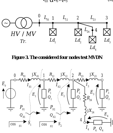
Let us consider the network depicted in Figure 3, which is a four-node test MVDN.
The general loads Ld1…Ld4 are represented using
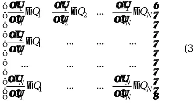
constant PQ models. Positive P (or Q) corresponds to the absorbed power by the load. Negative P (or Q) corres- ponds to the injected power in the network (i.e., the gene- ral load is really a generator). The per-phase equivalent circuit is shown in Figure 4.
The lines L01…L24 are modeled using the RL-direct
sequence equivalent circuit [15], but the shunt admittan- ces are neglected. The node 0 represents the MV busbar, which is regulated at a constant voltage value E0 by the
AVR of the OLTC. This reference voltage coincides with the rated value E0=Vn 3.
Because the busbar is regulated at E0, we can char-acterize the generic node i using the difference V0i be-
tween the magnitude of the busbar voltage and the node voltage Ei. In other words, we can write:
0i 0 i
V =E −E (4)
In radial networks, (4) can be calculated as the sum of the voltage differences between adjacent nodes from the ith node toward the MV busbar. For example, if i=3 (see Figure 4), (4) becomes:
03 0 3
V =E −E (5)
1
Ld Ld2 Ld3
4
Ld
01
L L12 L23
24
L
0 1 2 3
4
/
HV MV
.
[image:3.595.307.538.435.707.2]Tr
Figure 3. The considered four nodes test MVDN
0
E
1
E E2 E3
4
E
01
R jX01 R12 jX12 R23 jX23
24
R
24
jX
0 1 2 3
4
1
P
1
Q PQ22
3
P
3
Q
4
P Q4
1
S
1 S
P
1 S
Q
1
cosS S2
2 S
P
2 S
Q
2
cosS
1 S
I IS2 I3
4
I
By adding and subtracting E1 and E2 in (5), we ob- tain:
(
) (
) (
)
03 0 1 1 2 2 3
01 12 23
V E E E E E E
V V V
= − + − + −
= + + (6)
where V03 is the sum of the voltage differences V01,
12
V and V23.
23
V can be calculated considering the network para- meters and the line power flows as follows:
23 2 3
23 3 3 23 3 3
23 3 3 3 23 3 3 3
3
23 3 23 3
3
= cos sin
cos sin
V E E
R I X I
R E I X E I
E
R P X Q
E
= − +
+ =
+ =
ϕ ϕ
ϕ ϕ
(7)
where cosϕ3, P3 and Q3 are the power factor and the
active and reactive (per-phase) powers of the load Ld3,
respectively. I3, R23 and X23 are the current,
resis-tance and reacresis-tance of the line L3.
Normally, the nodal voltages are close to the rated voltage En. Applying this assumption to (7) leads to:
23 3 23 3 23
n
R P X Q
V
E
+
≅ (8)
Similarly, considering nodes 1 and 2, we can write:
12 1 2
12 2 2 12 2 2
12 2 2 2 12 2 2 2
2
12 2 12 2
cos sin
cos sin
S S
S S
S S
n
V E E
R I X I
R E I X E I
E
R P X Q
E
= −
= +
+ =
+ ≅
ϕ ϕ
ϕ ϕ
(9)
where PS2 and QS2 are the active and reactive powers
through the section S2 and cosϕS2 is the power factor
for the same section. For PS2 and QS2, we can write:
2 2 3 4 23 24
S R R
P =P + + +P P P +P (10)
2 2 3 4 23 24
S X X
Q =Q +Q +Q +Q +Q
(11)
where PR23 and PR24 are the power losses in R23 and
24
R , while QX23 and QX24 are the reactive powers
absorbed by X23 and X24. These active and reactive
losses are negligible compared to the load powers. Ap-plying this assumption to (9), (10) and (11) leads to:
2 2 3 4
S
P ≅P + +P P (12)
2 2 3 4
S
Q ≅Q +Q +Q (13)
and:
(
)
(
)
12 2 3 4 12 2 3 4
12
n
R P P P X Q Q Q
V
E
+ + + + +
≅ (14)
Finally, the voltage difference V01 is:
01 1 01 1 01 0 1
S S
n
R P X Q
V E E
E
+
= − ≅ (15)
where:
1 1 2 3 4
S
P ≅ + + +P P P P
(16)
1 1 2 3 4
S
Q ≅Q +Q +Q +Q (17)
are the powers through section S1.
Using (6) with (15), (9) and (8), we can say that V03
is a function of all loads and active and reactive powers, i.e., P1…P4 and Q1…Q4. The same observation is valid
for E3:
(
)
3 0 03 0 01 12 23
E =E −V =E − V +V +V (18)
because E0 is constant. In other words, we can write:
(
)
3 1,..., 4, 1,..., 4
E = f P P Q Q (19)
Equation (19) shows that an active/reactive power variation (in the general j node) that is defined as:
0 f
j j j
P P P
∆ = − (20)
0 f
j j j
Q Q Q
∆ = − (21)
where Pjf ( f j
Q ) and Pj0 ( 0 j
Q ) are the final and ini-tial power values, respectively, produces a voltage varia-tion in node 3 that is defined as:
0
3 3 3
f
E E E
∆ = − (22) In this treatment, we only consider the reactive power variations (i.e., ∆ =Pj 0) because we assume that only the reactive power can be used to control the node voltages.
The variation ∆E3 can be calculated by linearizing
(19) and considering only the reactive power variations. In particular, we can write:
3 3
3 1 2
1 2
3 3
3 4
3 4
E E
E Q Q
Q Q
E E
Q Q
Q Q
∂ ∂
∆ = ∆ + ∆ +
∂ ∂
∂ ∂
+ ∆ + ∆
∂ ∂
(23)
The terms ∂Ei ∂Qj in (23) indicate the “gain” from the voltage variation ∆Ei in node i when a reactive
power variation ∆Qj occurs in node j. In other words,
they are sensitivity terms.
3 01 12
2
3 01 12 23
3
3 01 12
4
n
n
n
E X X
Q E
E X X X
Q E
E X X
Q E
∂ = − + ∂
∂ = − + + ∂
∂ = − + ∂
(24)
Substituting equation group (24) into (23) has important implications. If we have a reactive injection in any node, i.e., ∆Qj <0 (in this case j=1...4), then ∆ >E3 0 in
node 3 (i.e., the voltage increases). Then, if we were to reduce the voltage in any node, we must abs- orb reactive power from the network (i.e., ∆Qj >0) by using, for example, the distributed generators.
If the above analysis that focuses on node 3 is extended to all network nodes, (23) has a general matrix relation- ship:
1 1 1 1
1 2 3 4
1 2 2 2 2 1
1 2 3 4
2 2
3 3 3 3 3 3
1 2 3 4
4 4
4 4 4 4
1 2 3 4
E E E E
Q Q Q Q
E E E E E Q
Q Q Q Q
E Q
E E E E E Q
Q Q Q Q
E Q
E E E E
Q Q Q Q
∂ ∂ ∂ ∂
∂ ∂ ∂ ∂
∆ ∂ ∂ ∂ ∂ ∆
∆ ∂ ∂ ∂ ∂ ∆
=
∆ ∂ ∂ ∂ ∂ ∆
∆ ∂ ∂ ∂ ∂ ∆
∂ ∂ ∂ ∂
∂ ∂ ∂ ∂
(25)
which in a compact form yields:
[ ]
∆ =E sQ[ ]
∆Q (26)where sQ is the reactive sensitivity matrix,
[ ]
∆Q isthe reactive power-variations vector and
[ ]
∆E is the nodal voltages vector.Calculating the partial derivatives contained in sQ ,
we have Equation (27).
After analyzing this form of (27), we can say that this matrix can be built using the following inspection rule:
“The element i j, is the arithmetic sum of the reac-tance of the branches in which both the powers absorbed by node i and node j flow multiplied by −1En ”.
For example, in (27), the element 2, 4 is
(
X01 X12)
En− +
because the powers delivered by node 2 and node 4 flow in branches 01 and 12.
3.3 The Choice of the Best Generator
The BG is the generator that has the greatest influence on node i, which is the node where the voltage exceeds the threshold.
Thus, after analyzing (25), we can say that the BG is the generator that maximizes the following product, which we call the “sensitivity product”:
i j j
E Q Q
∂ ∆
∂ (28) For example, if the node with a voltage that exceeds
max
V is i=2 and the BG is connected to node j=4, the sensitivity product
(
∂E2 ∂Q4)
∆Q4 is the highest compared to the other products contained in row 2 of the sensitivity matrix. In addition, in order to choose the BG, it is necessary to evaluate the single products (28) of the row that represents node i. Thus, the value ∆Qj isneeded and is acquired as the GCC polls the GRTUs, as stated previously.
The procedure described above suggests a way of de-fining the “sensitivity table”
[ ]
TS that contains thesin-gle sensitivity products. For the MVDN represented in Figure 4,
[ ]
TS takes the following form1 1 1 1
1 2 3 4
1 2 3 4
2 2 2 2
1 2 3 4
1 2 3 4
3 3 3 3
1 2 3 4
1 2 3 4
4 4 4 4
1 2 3 4
1 2 3 4
E E E E
Q Q Q Q
Q Q Q Q
E E E E
Q Q Q Q
Q Q Q Q
E E E E
Q Q Q Q
Q Q Q Q
E E E E
Q Q Q Q
Q Q Q Q
∂ ∂ ∂ ∂
∆ ∆ ∆ ∆
∂ ∂ ∂ ∂
∂ ∆ ∂ ∆ ∂ ∆ ∂ ∆
∂ ∂ ∂ ∂
∂ ∂ ∂ ∂
∆ ∆ ∆ ∆
∂ ∂ ∂ ∂
∂ ∂ ∂ ∂
∆ ∆ ∆ ∆
∂ ∂ ∂ ∂
(29)
Row i represents the node in which we want to co- ntrol the voltage, and column j represents the nodes in which we can control the reactive power. The BG is the generator connected to node j that has the maximum absolute value of the sensitivity product in position i j, . By finding the maximum sensitivity product in row i,
01 01 01 01
01 01 12 01 12 01 12
01 01 12 01 12 23 01 12
01 01 12 01 12 01 12 24
1
Q
n
X X X X
X X X X X X X
s
X X X X X X X X
E
X X X X X X X X
+ + +
= −
+ + + +
+ + + +
we automatically choose the BG because the location corresponds to column j of the maximum sensitivity pr- oduct.
It is clear that, for a general network with N nodes, the sensitivity table takes the following form:
1 1 1
1 2
1 2
2 1 1
1 1
...
... ... ...
... ... ... ...
... ...
N N
N N
N N
E E E
Q Q Q
Q Q Q
E Q Q
E E
Q Q
Q Q
∂ ∂ ∂
∆ ∆ ∆
∂ ∂ ∂
∂ ∆
∂
∂ ∂
∆ ∆
∂ ∂
(30)
It is important to note that, if it is not possible to regulate the reactive power (e.g., if in that node there is a load or a non-controllable generator) in a node j, then
0
j
Q
∆ = and, consequently, the sensitivity product in the position i j, of the sensitivity table is 0.
Comparing (29) with (25), we can say that each ele- ment i j, of
[ ]
TS represents the line-to-ground voltagevariation in node i when a reactive power variation occurs in node j.
In the following section, a numerical example of the sensitivity method application is shown.
4. Application of the Proposed Method
The network considered in this numerical application is represented in Figure 5.
During normal network operation, we have four ge- nerators and eight loads. The generator and load charac-teristics are summarized in Table 1 (S is the apparent power) and Table 2, respectively (three-phase powers are represented in these tables).
We suppose that the generators normally operate with a unitary power factor (i.e., no reactive power is injected in the nodes).
The per-kilometer reactance of the cable lines is x= 0.17Ωkm, which is a typical value for Italian MVDNs. The line lengths and parameters are summarized in Ta-ble 3.
Let us suppose that each generator is connected to its GRTU that measures the nodal voltage and communicates with the GCC. Moreover, let us suppose that G5 cannot
regulate the reactive power because it is not designed for this purpose. The MV busbar is regulated at the rated voltage (1 p.u.), which is 20 kV (line-to-line). In this example, the voltage threshold Vmax is 1.05 p.u.
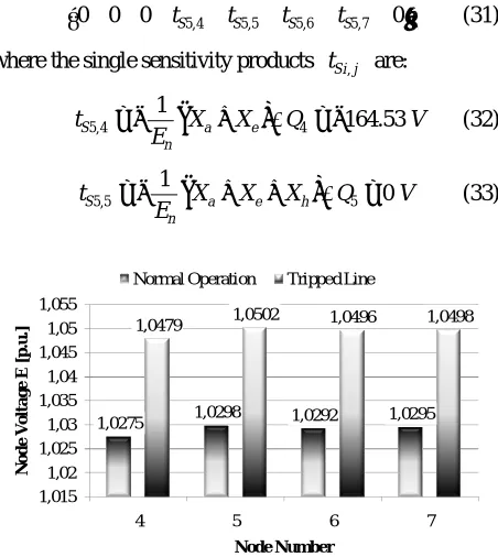
Using load-flow software, we calculated the voltage E in the generator nodes (nodes 4, 5, 6, and 7) for normal network operation. The results are shown in Figure 6 (Normal Operation).
0 1
2
3
4
5 6 7
8
a b
c d
e f g
h l
m
n
i q
p
o
7
G
5
G
6
G
4
G bl
cl
dl
gl ol
pl nl ml
,
B ref
V
B
[image:6.595.86.280.151.256.2]V
Figure 5. The network considered in the numerical applica-tion
Table 1. Loads characteristics
Load S [MVA] cos P [MW] Q [MVAR]
bl, nl 2 0.95 1.9 0.62
cl 7 0.92 6.44 2.74
dl 3 0.92 2.76 1.18
gl 2.08 0.95 1.99 0.62
ml 2.58 0.93 2.4 0.94
ol 1.98 0.96 1.9 0.57
pl 1.5 0.92 1.38 0.59
Table 2. Generators characteristics
Generator P [MW]
G4 6
G5 1.75
G6 4.5
[image:6.595.308.537.236.350.2]G7 3.75
Table 3. Lines parameters
Line Name L [km] X [Ω]
a, l, q 2 0.34
b, f, g, i, m, n 1 0.17
c, d, o, p 0.5 0.085
e 15 2.55
h 5 0.85
If line b trips (e.g., due to a fault), loads bl, cl and dl are cut off from the supply, which causes the voltage to increase in the network. In particular, if the load-flow is re-computed to take into account the new network con-figuration, we obtain the results shown in Figure 6 (Tripped Line).
It is important to note that, if the voltage exceeds the maximum threshold Vmax in node 5, the GRTU
con-nected to G5 sends the VTO signal to the GCC that must
choose the BG using the sensitivity table.
[image:6.595.312.537.481.562.2]last poll are those summarized in Table 4, which also contains the corresponding power factors cosφ. To cal-culate the sensitivity table, we need the single-phase powers. Therefore, the reactive powers shown in Table 4 have to be divided by three. It is important to note that the reactive powers calculated this way correspond to
j
Q
∆ because Qj0 is zero (see (21)). The ∆Qj values
are shown in Table 5.
The voltage exceeds the threshold in node 5. Thus, we only consider the fifth row of the sensitivity table. According to the inspection rule mentioned above, this row is as follows:
5,4 5,5 5,6 5,7
0 0 0 tS tS tS tS 0
(31)
where the single sensitivity products tS i j, are:
(
)
5,4 4
1 Δ
164.53
S a e
n
t X X Q V
E
= − + = − (32)
(
)
5,5 5
1
Δ 0
S a e h
n
t X X X Q V
E
= − + + = (33)
1,0275 1,0298 1,0292 1,0295
1,0479 1,0502 1,0496 1,0498
1,015 1,02 1,025 1,03 1,035 1,04 1,045 1,05 1,055
4 5 6 7
N
o
d
e
V
o
lta
g
e
E
[
p
.u
.]
Node Number
[image:7.595.339.534.85.180.2]Normal Operation Tripped Line
[image:7.595.61.287.235.488.2]Figure 6. Load-Flow results with the Network Normal Op- eration
Table 4. Reactive powers absorbable by the generators
Generator Q[MVAR] cosφ
G4 1.97 0.95
G5 0.00 1
G6 0.91 0.98
G7 1.23 0.95
Table 5. Reactive Power Variations in the Generator Nodes
Generator ∆Qj[MVAR]
G4 0.66
G5 0.00
G6 0.30
G7 0.41
(
)
5,6 6
1
Δ
98.65
S a e h
n
t X X X Q
E V
= − + +
= −
(34)
(
)
5,7 7
1 Δ
133.07
S a e h
n
t X X X Q
E V
= − + +
= −
(35)
The maximum sensitivity product (in absolute value) corresponds to generator 4, (i.e., j=4). Thus, the BG is G4.
Equation (32) provides important information. If G4
performs the considered reactive power variation, the line-to-ground voltage variation in node 5 is:
5
ΔE = −164.53V → −0.0142 p u. . (36) Then, considering (22) (rewritten for node 5), and
0
5 1.0502 . .
E = p u from Figure 6, we can say that the voltage value after the reactive power variation is:
0
5 5 Δ 5 1.036 . .
f
E =E + E = p u (37)
which is less than the voltage threshold Vmax.
Equation (37) shows the theoretical result obtained using the proposed method. We checked this value using load-flow software:
5 1.034 . .
f load flow
E = p u (38)
The percentage error between (38) and (37) is:
5 5
%
5
100 0.19 %
f f
load flow f
load flow
E E
ε
E
−
= ⋅ = − (39)
which is negligible and demonstrates the validity of the proposed approach.
5. Conclusions
The proposed sensitivity method allows the voltage wi- thin network acting on single generators to be regulated by choosing the most effective generator on the contr- olled node (i.e., the Best Generator). This is a very im-portant feature in grids that have distributed generation (e.g., in a Smart Grid context).
The proposed method uses a topological approach. Mo- reover, the sensitivity table can be constructed automati-cally.
In addition to the BG choice, the proposed method al- so evaluates the voltage in all network nodes after a reac-tive power variation.
[image:7.595.57.288.549.622.2] [image:7.595.58.286.657.723.2]When a generator is switched during RPA, it works wi- th a non-unitary power factor; the reactive power flow in- creases along the lines and increases the power loss [16].
This phenomenon is negligible in HV networks beca- use the line resistance is typically smaller than the line reactance, but is important to consider in MV networks.
Therefore, if network analysis reveals that the RPA- switching produces high losses, voltage control using the reactive power variation must only be used for temporary voltage variation mitigation (i.e., during emergency con-ditions).
The possible future develops of this work could be fo-cused on the optimization of the forecasted power-time profiles of the loads and generators applying both the se nsitivity approach and distributed voltage measurement.
REFERENCES
[1] R. Marconato, “Electric Power Systems,” Vol. 2, CEI, Milano, 2008.
[2] P. Kundur, “Power System Stability and Control,” McGraw- Hill, New York, 1994.
[3] Y. Rosales Hernandez and T. Hiyama, “Distance Measure Based Rules for Voltage Regulation with Loss Reduc-tion”, Journal of Electromagnetic Analysis and Applica-tions (JEMAA), Vol. 1, No. 2, June 2009, pp. 85-91. [4] F. Saccomanno, “Electric Power Systems”
Wiley-Interscience IEEE Press, Piscataway, 2003. [5] G. Andersson, “Modeling and Analysis of Electric Power
Systems” Lecture 227-0526-00, ITET ETH Zürich, Zürich, 2008.
[6] Y. Abdel-Rady, I. Mohamed and E. F. El-Saadany “A Control Scheme for PWM Voltage-Source Distributed- Generation Inverters for Fast Load-Voltage Regulation and Effective Mitigation of Unbalanced Voltage Distur-bances” IEEE Transactions on Industrial Electronics, Vol. 55, No. 5, May 2008, pp. 2072-2084.
[7] P. M. S. Carvalho, P. F. Correia and L. A. F. M. Ferreira, “Distributed Reactive Power Generation Control for Vol-
tage Rise Mitigation in Distribution Networks,” IEEE Transactions on Power Systems, Vol. 23, No. 2, 2008, pp. 766-772.
[8] P. N. Vovos, A. E. Kiprakis, A. R. Wallace and G. P. Harrison, “Centralized and Distributed Voltage Control: Impact on Distributed Generation Penetration,” IEEE Transactions on Power Systems, Vol. 22, No. 1, 2007, pp. 476-483.
[9] P. M. Anderson, “Power System Protection,” IEEE Press, Piscataway, 1999.
[10] N. Mohan, T. M. Undeland and W. P. Robbins, “Power Electronics: Converters, Applications, and Design”, Wiley, 1995.
[11] M. H. Rashid, “Power Electronics Handbook”, Academic Press-Elsevier, 2007.
[12] L. L. Grigsby, “Electric Power Generation, Transmission and Distribution,” CRC Press-Taylor & Francis Group, Boca Raton, 2006.
[13] F. A. Viawan and D. Karlsson, “Coordinated Voltage and Reactive Power Control in the Presence of Distributed Generation,” PES General Meeting - Conversion and De-livery of Electrical Energy in the 21st Century, IEEE, Pittsburgh, 2008, pp. 1-6.
[14] S. Corsi, “Wide Area Voltage Regulation & Protection” 2009 IEEE Bucharest Power Tech Conference, Bucharest, June 28 -July 2, Bucharest, pp. 1-7.
[15] A. Gandelli, S. Leva and A. P. Morando, “Topological Considerations on the Symmetrical Components Trans- formation”, IEEE Transactions on Circuits and Systems I: Fundamental Theory and Applications, Vol. 47, No. 8, August 2000, pp. 1202-1211.
[16] H. M. Ayres, L. C. P. da Silva, W. Freitas, M. C. de Alm- eida and V. F. da Costa, “Evaluation of the Impact of Distributed Generation on Power Losses by Using a Sen-sitivity-Based Method,” IEEE Power & Energy Society General Meeting, Calgary, 2009, pp. 1-6.
[17] A. Kishore and E. F. Hill, “Static optimization of Reac-tive Power Sources by use of Sensitivity Parameters”,