Active Queue Management within Large Scale Wired Networks

(1)

doi:10.4236/ijcns.2011.44029 Published Online April 2011 (http://www.SciRP.org/journal/ijcns)

Active Queue Management within Large-Scale

Wired Networks

Ping-Min Hsu1, Chun-Liang Lin1

,

Ching-Han Yu2 1

Department of Electrical Engineering, National Chung Hsing University, Taichung, Chinese Taipei

2

Department of Electrical Engineering, National Taiwan University, Chinese Taipei

E-mail: [email protected]

Received March 3, 2011; revised March 24, 2011; accepted March 30, 2011

Abstract

Signal transmission control protocol sources with the objective of managing queue utilization and delay is actually a feedback control problem in active queue management (AQM) core routers. This paper extends AQM control design for single network systems to large-scale wired network systems with time delays at each communication channel. A system model consisted of several local networks is first constructed. The stability condition guaranteeing overall stability is subsequently derived using Lyapunov stability theory. The results developed have been successfully verified on a network simulator.

Keywords:Large-Scale System, Network Control, Stability, Time Delay

1. Introduction

Traffic characterization and modeling are generally rec-ognized as two important steps toward analysis and con-trol of network transmission performance. With the aid of the characterized model, control theory can be effi-ciently applied in solving the congestion control problem. There have been various delayed differential equation models developed in [1-3], in which the fluid-flow model utilized in [1] was previously proposed in [2]. Those characterized data traffic as fluid used a set of differen-tial equations to describe the Active Queue Management (AQM) policy and the router queuing process. In [4], the end-to-end congestion control mechanisms were em-ployed in transmission control protocol (TCP) flow con-trol.

While a bunch of research focusing on modeling and analysis of network control systems have been published, most approaches addressed the issue for a single sender- receiver network connection [5].

This paper is motivated by the requirement of an ap-proach for modeling and stabilization of large-scale communication networks. An extension of the fluid- based model in wireless networks was proposed in [6,7], in which their parameters for representing the probability of data transmission failure was applied in system de-velopment. A system for mixed wired and wireless net-works was concerned in [6], in which a more general

fluid-based model compared with that in [1] was

pro-posed. A robust H_ controller design was proposed in

[7], in which the stability analysis was conducted by Lyapunov theory and modern control theory was ex-tended to deal with the network congestion problem. Fur- thermore, linear matrix inequalities were proposed in control design and less oscillation under TCP was achieved. Packet dropout not only affects stability in data transmission, but also plays an important role in the net-work control systems. The authors in [8-10] have inves-tigated stability for the network control systems with packet dropout.

To the best of the authors’ knowledge, while the Lya-punov stability theory has been widely applied to the stability analysis of large-scale systems [11-13], investi-gation for stability of the large-scale network control systems (LWNCSs) are quite rare. This motivates this research. The presented work shows that an appropriate control design based on an appropriate Lyapunov func-tional ensuring asymptotic stability of the LWNCS can be constructed when there are a large number of signal flows.

The major contributions can be summarized as fol-lows.

1) A control strategy for congestion control in the

large-scale wired network is constructed.

2) All local networks are interconnected according to

(2)

works mutually affect each other within a wired network scheme is modeled via a particular form of the dropping probability.

An example is given to demonstrate validity of the re-sult using the network simulation platform NS2 [14].

2. Modeling of Large-Scale Wired Network

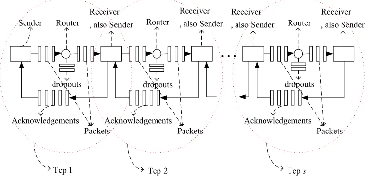
The large-scale wired network under consideration is as

illustrated in Figure 1, which consists of s locally

wired networks within TCP under random early detec-tion (RED). In each TCP loop, signal packets are trans-mitted from a sender to a receiver, which is also the sender to next TCP loop. Furthermore, they are

sequen-tially passed from TCP1 to TCPs. Some packets are

dropped in the congested router under RED, in which the dropping probability is computed by the proposed

con-troller. Regarding the topology illustrated in Figure 1,

the current dropping probability not only determines the seriousness of transmission congestion in the present router, but also affects those in other congested routers in the large-scale wired network.

Referring to [1], a simplified version of a fluid-flow model of TCP behavior involving the key network vari-ables could be modeled as

 

_{ }

 

_



_{ }

 

_





 



 

0

1 _,

2 0

W t R t W t

W t p t R t

R t R t R t

W W



  

 



(1)

 

     

 

     





0

, 0 ,

max 0, , 0

N t W t R t C q q q

q t

N t W t R t C q

 



  _ _



 0 (2)

where is the average TCP window size (packets),

is the average queue length (packets/sec), W

q R t

 

is

the round trip time (RTT), is the link capacity

(packets/sec), N is the loading factor (the number of TCP

sessions), and

C

[0,1]

p is the probability of packet

mark. The queue length q



0,q_m



and the window size



0, _m



W W where q_m and W_m denote the buffer

ca-pacity and the maximum window size respectively. Let

 

R t denote the RTT for t0 and is assumed to be

 

p

R t q t C T (3)

where Tp is the fixed propagation delay and q t

 

C

models the queuing delay. One is referred to [1] for the details of the mathematical modeling of the fluid-flow model of TCP.

Suppose that each dynamic model of TCP constructs a sub-network, which belongs to an interconnected bottle-neck network, then a large-scale wired network

com-posed of s interconnected bottleneck networks Si,

1, 2, ,

i  s can be shown as in Figure 2, where

 

, 1, ,

i i i ip

R t q t C T i  s , with being the

propagation delay for TCPi and

ip T

1 2

( ) ( ) q ( )t

i i i

si

q t q t 

( )t q

  . From (1) and (2), the large-scale linearized

differential equations can be written in the matrix form as

 













2 2

2 2 0

0 0 2

0 0

0

2 2

0 0

0

δ δ

1

δ

δ , (4)

2

1 δ

0

1 _δ

, 1, 2, ,

δ

0 0

i

i i i

i i i i

i io

i

i i

i

i i

i i i i

i i

w t

q t

N

R C w t

R C R C

p t R N

N q t

R R

N

w t R

R C R C i s

q t R

 

 

 

 

 

 

 _{ } _{ }



 

_ _ _{ } _

 __ __{ } _

   

 



 _{ } _ _

 

_ _  



 

 

 

 

 



with each sub-network being interconnected through



Router Sender

Receiver , also Sender

Packets Acknowledgements

Router

Receiver

, also Sender Router

Receiver , also Sender Receiver

, also Sender

Tcp 1 Tcp 2 Tcp s

Packets Acknowledgements Packets

Acknowledgements

[image:2.595.321.538.345.483.2]

dropouts dropouts dropouts

[image:2.595.111.487.523.703.2]

(3)

 w1  

1 w 1 p 1 q 1 q 1 1 R

 w2 

2 w 2 p 2 q 2 q 2 1 R

TCP 1

TCP 2

     1 2 s w s w s p s q s q

TCP s

         routed packets data packets

Congested Router 1

Congested Router 2

Congested Router s

11 q 1 s q 12 q 2 s q 1s q ss q AQM control law AQM control law  1 2 1 2 1 1 R 2 1 R 1 R s e 2 R s e   1 1 R 1 C 2 C 1 N 2 N 2 1 R   s N s C 1 s R  AQM control law s R s

e 1

[image:3.595.67.277.79.259.2]

s R 1 s R 21 q 22 q 2s q

Figure 2. Block diagram of the large-scale wired network.













 









0 0 0 0 1 0 0 1 0

3 3 3

0

2 3 3

0

δ , d δ

δ d

2 δ d

2 δ d , , 1, 2

i

s

i io pi j ij j ij

s

i R i pi j ij i

i _R i i i

p t R K q q t h

p p t v v K d t

v

N w t v v R C

v

N q t v v R C i j

v         _   _         _        _   





 u ,s (5)

where _ij is the transmission time between the bottleneck

networks h S_i and Sj ; δwiwiwi0 , δqi qiq0,

0

j j

q q q

   , and ₀; ₀ ₀ _i₀ denoting

our operating point; _i and

δp_ip_ip_i



w_i , ,q p



q q_j

i

N

denote data packets

belonging to the ith and jth sub-networks respectively;

i denotes the ith expected TCP sending window; i

denotes the link capacity; denotes the number of the

ith TCP sessions;

w C

0 0

i i ip

R q C 

max

p

T ; p_i is the

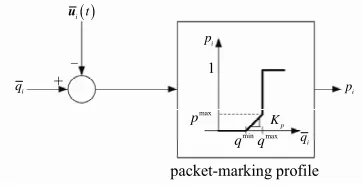
probabil-ity of packet mark; RED consists of a proportional

con-troller and packet-marking profile, shown as in Figure 3,

where , and are configurable

parame-ters and _pi denotes the slope of the active queue

management control law which computes _i as the func-

tion of the measured queue length

mi q n K max q p i

q by the AQM

pol-icy; _ij is the flow distribution ratio from the

bottle-neck network

d

j

S to S_i. If q ti

 

is bounded by

and , the packet-marking probability is given by

min q max q









 









0 0 0 0 1 0 1 3 0 3 3 0 2 0 3 3 0 δ

δ d d

2 δ d 2 δ d i i i s

i pi ij j ij

j

s

i pi ij i

R j i i R i i i i R i i

p K d q q t h

p t v v K t

v

N

w t v v

v R C

N

[image:3.595.333.514.80.173.2]

q t v v v R C   _      _   _        _         _  _





u min q max q max p i p 1 p K i q i p   i t u -+ i q packet-marking profile

Figure 3. RED drop function.

The form of (5) is determined based on the following considerations.

1) While each sub-network is interconnected through

(5), the feedback signal applied for the controller is treated as the combination of all the queue lengths in the large-scale network. Thus, the term





0

1 δ

s

ij j ij

jd q  q th 



in (5) was claimed. It

was further multiplied with Kpi, which denotes

the slope of the active queue management control law.

2) The term





0

δ d

i i

R _v p t v v 

 _ 



denotes the differ-

ence between the current and delayed values of the

dropping probability adopted in the ith TCP.

Con-sidering the fluid-flow model, the current queue length variation is affected by the delayed dropping probability while the current one is applied in real world. Considering this fact, while constructing (5),

the term





0

δ d

i i

R _v p t v v 



 





is added.

3) pi0 is added to cancel pi0 while computing

where δ i

p

0

i i i

p p  p.

4) Additional terms in the AQM controller law are

added to obtain the transformed system (6) with the controller (7).

5) Now, substituting δp t Ri



, i0



, defined by (5), into

(4) gives a new system. Based on (4), a large-scale

wired network system consisting of s local

net-works can be expressed in the state-space repre-sentation as follows

 

, 1, 2, ,

i ii i i i

x t A x t B u t i  s (6)

where xi

 

t  δw ti

 

δq ti

 

T,

2 0

0 0

2Ni

 0 1 i i ii i i i R C N R R   , 2 0 2 2 0 i i i i R C N           

B , and

            A 1

( ) s ( ) ( ( )), , 1, 2, ,

i ij j ij i i

j

t F x t h t i j





    

u u s (7)

with Fij  0 K dpi ij and ui

 

t  Kixi

 

t being

[image:3.595.75.284.289.383.2]

(4)

 







 















0 0 0 0 0 1 0 3 0 3 3 0 2 0 3 3 0 δ d

2 _δ _d

2 δ d i i i s

i i pi ij i i

j i R i i R i i i i R i i

t K d q t p

p t v v v

N

w t v v

v R C

N

q t v v v R C                _         _  





u u

Equation (6) represents the linearized system of the large-scale wired network while considering coupling effects induced by the locally wired networks. The term

implies the dropping probability while concerning

the interconnection of local networks. The term i

 

t

u

 

i t

u

is to be determined in the stability analysis. Equation (7) is

treated as the control input such that p t_i

 

u_i

 

t p_i₀

is applied as the dropping probability.

 

i t

u can be derived in the following steps:

Step 1) Consider (5), which models how local net-works may mutually affect each other in the large-scale wired networking environment.

Step 2)Substitute δp t R_i



, _i₀



into (4) and use xi 

to obtain system of (6) with the controller (7). i



i0

tR

x



From (6) it is easily seen that is controllable.

The action of the AQM control law is to mark packets as

a function of the measured queue length q. The plant

dynamics given by (6) relates reveals the packet-marking probability dynamically affects the queue length.



A B_ii, _i

Now, let the set of feasible operating conditions





0 0, m

q  q , w_i₀



0,W_m



, and p_i₀

 

0,1 . Assume

that δw_i, δqi and δpi are continuously differentiable

on



Ri0, 0



, i.e.

i W w   b

v   

 , δ i q q b v  _ _{ }  , δ  _

 i p p

b

v   ,   v



Ri0, 0



.

Therefore





0 0 0 δ d

i i W

R _v w t v v b R 

 _ _ 



i ,





0

δ d

i i q

R _v q t v v b R 



  



i ,





0

δ d

i i p

R _v p t v v b R 



  



i .

Furthermore

 



 



 





 

2 0 1 1 0 s s

i i i pi ij i pi ij i

j j

i i i

t t K d t K q d

p g t t

 

  

 



u u u u

u t (8) where

 













0 0 0 3 0 3 3 0 2 0 3 3 0 0

2 _δ _d

2

δ d

+ δ d

i

i _R i

i i i i R i i i R N

g t w t

v R C

N

q t v v

v R C

p t v v

v              _ 



v v

It is seen that gimg ti

 

gim with

3 2 3 0 2 i im W i i N g b R C  2 0 2 3 0 2 i

q i bp i i

N

b R

R C

  . The gain Kpi is chosen as









0 0 1 0 0 1 1

, when 0,

1, 2, ,

1 _{, otherwise,}

i im i

s ij j pi i im s ij j p g q d

K i s

p g q d    _ _       _   



 u (9)

This ensures u_i

 

t _i



u_i

 

t



 0, u_i

 

t .

With regard to the above system one can ensure that

 

i

  , i1, 2, , s satisfy

 



 



 

2 _{, ,}_{1, 2, ,}

i i t i t i i t i t R i s

 u u  u u    (10)

From (8) and (9), the gain reduction tolerance is given

by s ₁

i Kpi j dij

 



_ 

where dij, j1, , s are chosen

1

such that s₁

iKpi



jdij .

3. Stability of LWNCS

The following theorem states the main result which cha-racterizes the stability condition for the LWNCS.

Lemma: For any scalar 0 and any real vectors

X and Y with appropriate dimension, then

T T _ T 1



   T

X Y Y X X X Y Y (11)

Theorem: The large-scale wired network system

de-scribed by (6), which satisfies (10), would be asymptoti-cally stable, if the state feedback control law of each sub-network is given by

 

1

 

, 1, 2, ,

2 T

i t   i i i i t i 

u B P x s (12)

where i  1  i i with i satisfying

2i 2 1i i 2 i 2 1i (13)

and T 0

i  i 

P P satisfies the following Riccati matrix

inequality:









T T 1 +1 0

ii i i ii i n i i i i i

i n s s         _   _  

A P P A P I B B P

I

(5)

in which 1 is a positive constant,  i  i(i i)2 4

and i: max



ji,j1, 2, , s



with ji satisfying

Proof: The stability analysis is derived around the

ori-gin δqiδwi0 of (4), i.e. the equilibrium point



q p0, i0,wi0



of the fluid-flow model. Regarding the

problem, we define an appropriate Lyapunov functional candidate as

1

, ,

T T

ij n ij i i ij i j

  

I F B B F  (15)

 

T

 

T

   

2

 

0 0

1 1

d d

ij

s s _t _t _t

T

i i i i i ij _{t h} j j i i i i

i j

t t  _        2  d

 

 

 _    _

 



 



V x x P x x x x x u (16)

for 1, 2, ,i



 s



. The set



q p0, i0,wi0



chosen as the

equilibrium point of the fluid-flow model corresponding

to TCPi is determined by

2

0 0

0 0 0 0

0 0 0

1

0, 0, , 1

2

i i

i i i i ip i

i i i i

w N q

p w C R T p

R  R  R    C 

It is obtained that Vi

 

0 0 while ui0 and

for . Taking differentiation with

re-spect to time t and using (6) while ignoring

and

 

0 i xi 

V xi0

   

T

1 0 0

s

i i

i





x x s₁ _i2

 

0 i





u gives

 





 



 



   



 



T T

1

2 2 T

1 1

T 1

T T

1 1

+2

s

i i i ii i i ii n i

i

s s

i i i i i ij j ij

i i

s

i i i i i

i s s

ij j j j ij j ij

i j

V t I t

t t t h

t t

t t t h t h



 

 

  

 

 _   _

 



 

 _   _





 _x _x _{A P} _{P A} _x

u x P B F x

x P B u

x x x x 

It is easily obtained from (11) that





 

















 









 

T T T T

1 1

T T T

1 1 1 T 1

T T 1 1 1

T 1

1

s s

j ij ij i i i i i i ij j ij

i j s s

j ij ij i i ij j ij

i j

i i i i

s s T

j ij ij i i ij j ij

i j s

i i i i

i

t h t t t h

t h t h

t t

t h t h

s t t



  

 



 



 _  





 _

 

 _   _

 







x F B P x x P B F x

x F B B F x

x P P x

x F B B F x

x P P x





 



 



 

T

1

T T

1

2 s _i _i _i _i _i

i s

i i i i i i i i i

t t

t P

  





 



x P B u

x P B B x t

(17)

Furthermore

   

T T

1 1 1

s s s

ij j j i i i

i j i

t t s t t

 

  





x x



x x

Therefore, it can be obtained that

 









 









T T 2

1 1

2

T T T

1 1 1

1

1 +

4

1 +

s

i i i ii i i ii i n i

i

T i i i i i i i i i

s s

j ij ij i i ij ij n j ij i j

t s s

t

t h t h

 

   

 



 



 _    

  _ _ _ 

  

  

 

 _  _

 







V x x A P P A I P

P B B P x

x F B B F I x

where  ₁ 0. After substituting (12) into (10), one

gets _

(18)

 



 



T T ₂ T

i i i t i i i i ix t i t i i i i

 x P B B P  x P B u t

From (12)-(15), it can be concluded that i.e.

 

T

 

T T T T

1 1 1 1

1 1

0

1 1

0 , ,

i s

i i i i

i i i i i i n is i i is is n

J

t t

diag  

 



 

 

 _  _

 

 

 _ _

 







V x

F B B F I F B B F I

(6)

where

 

T

 

T





T





T,

1 1

i t xi t x thi  xs this 











T T

1 +1 0

i ii i i ii is n  i i i i  i si n

J A P P A P I B B P I

and T T

1, ,

ij n ij i i ij i j

 I F B B F   and _i satisfies

(13). This completes the proof.

4. Design Process

Control design procedure is given bellows to summarize the previous analysis.

Step 1) Set parameters of the LWNS including i,

i, i0, ip, w, , and

C

N R T b b_q bp. The system model of (6)

is then constructed.

Step 2) Consider the model defined by (6) and (7) with

the positive constant 1, the parameter ij is chosen to

satisfy (15).

Step 3) Find ai, gim, i, i, i and to solve for

the Riccati matrix inequality (14). The solution can be calculated by transforming (14) into

T ₀

i i 

P P

linear matrix inequalities and solved via the available computational software.

Step 4) Obtain the control gain T ₂

i i i i

K B P . The

AQM control law u_i

 

t is determined by (7) with

 

i t   i i t

u K x .

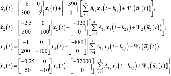
5. Illustrative Example

Consider a large-scale wired network described by (4)

with q0175 packets, N160, N250, N320,

4

N 5 , , 20 , ,

40 ,

10

R

0.1 s C

0.2 s



1 3, 750

0.1 s R

R  300.1 s

R   packets/s,

pack-ets/s, 2

4,

C  000

3 4,0

C  00 packets/s, 4 packets/s,

and 1

4, 000



C 0.001

  . The large-scale wired network consists

of four sub-networks described, respectively, by

 







 



 







 



 







 



 

4

1 1 1 1 1 1

1 4

2 2 2 2 2

1 4

3 3 3 3 3 3

1

4

8 0 390

,

300 5 0

2.5 0 320

,

500 100 0

1 0 889

,

200 100 0

0.

j j j

j

j j j

j

j j j

j

t t A t h t

t t A t h

t



   

   

_ _ _ __    _



     

 

2 t

t

 

   

_ _ _ __    _



     

   

   

_ _ _ __    _



     

 





x x x u

x x x

x x x u

x

 





u

 





4

4 4 4 4

1

25 0 32000

50 10 0 j j j

j

t A t h

 

4 t

 

  _  _ _{ }

 

 _   

 x   



x u 

Select  ij 0.04

W p q

b b b

for each and

as-sume so that



,

1, 2, 3, 4

i

1m 40

g 



200

 g2mg3m

. Referring to [1],

4m g

 20 w_i₀R C_i₀ i Ni and

. From

2

0 0

i i

w p 2 _ip_i₀g_im q₀ then ,

2 3 4

1

 0.2 0.1

    , and  1 2340.4 are

chosen to meet (13). Solving for the Riccati matrix ine-quality (14) gives

1 2

3 4

0.321 0.017 0.028 0.006

,

0.017 0.002 0.006 0.003

0.0009 0.0007 0.00004 0.00004

,

0.0007 0.0018 0.00004 0.0042

   

_ _ _ _

   

  

_ _ _

  

P P

,

  

and the corresponding control gain matrices are obtained as K1 



27.07 1.45



, K2 



9.22 2.01



,





3 2.77 2.05 , and

K K4 



2.16 1.92



re-spectively. The size of the packet is assumed to be 500 bytes.

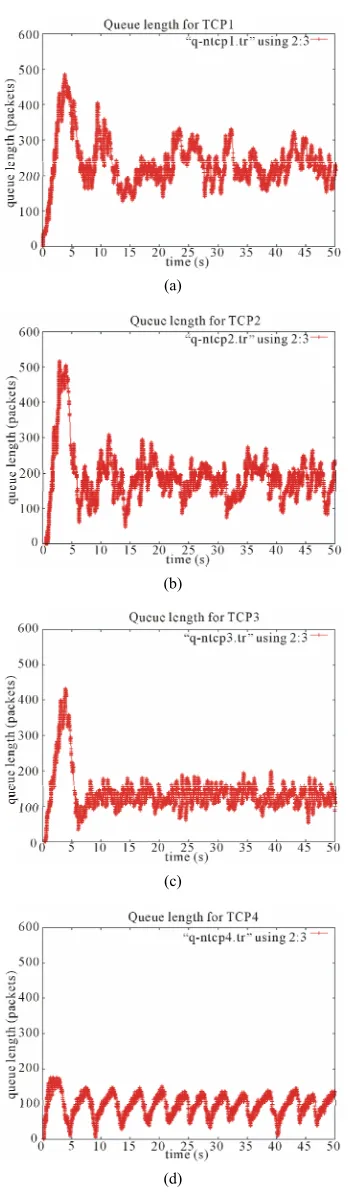
The numerical experiments are conducted on a net-work simulator-NS2 [14]. The simulation results with the

[image:6.595.153.444.339.469.2]

chosen parameters show satisfactory performance of the queuing response in the presence of random delays, see

Figure 4. It is found that larger TCP flows cause higher

link utilizations, but with larger queuing delays.

The results for the case of N1100, N250,

3 20

N  , N45 are displayed in Figure 5. As it can

be seen from Figure 5(a), large queue oscillations may

cause considerable variations in the RTT of packets for the corresponding sub-network. However, with the pro-posed controllers, the network still remains to be stable when it holds a large number of data flows.

6. Conclusions

(7)

(a)

(b)

(c)

[image:7.595.84.257.70.665.2]

(d)

Figure 4. Transient response of queueing with N160, 2 50, 3

N  N 20 and 4 . (a) Queue size for TCP1;

(b) Queue size for TCP2; (c) Queue size for TCP3; (d) Queue size for TCP4.

5 N 

(a)

(b)

(c)

(d)

Figure 5. Transient response of queueing with N1100, 2 50

N  , N320 and N45. (a) Queue size for TCP1,

[image:7.595.337.511.72.673.2]

(8)

presented. The simulation study conducted on the NS2 has been verified successfully.

7. Acknowledgements

This research was sponsored by National Science Council, Taiwan under the grant NSC No. 95-2221-E-005-017.

8. References

[1] C. V. Hollot, V. Misra, D. Towsley and W. B. Gong, “Analysis and Design of Controllers for AQM Routers Supporting TCP Flows,” IEEE Transactions on Auto-matic Control, Vol. 47, No. 6, 2002, pp. 945-959.

doi:10.1109/TAC.2002.1008360

[2] V. Misra, W. B. Gong and D. Towsley, “Fluid-Based Analysis of a Network of AQM Routers Supporting TCP Flows with an Application to RED,” Proceedings of ACM Special Interest Group on Data Communication, Stock-holm, 28 August-2 September 2000, pp. 151-160. [3] P. F. Quet and H. Ozbay, “On the Design of AQM

Sup-porting TCP Flows Using Robust Control Theory,” IEEE Transactions on Automatic Control, Vol. 49, No. 6, 2004, pp. 1031-1036.doi:10.1109/TAC.2004.829643

[4] B. A. Chiera and L. B. White, “A Subspace Predictive Controller for End-to-End TCP Congestion Control,” Proceedings of Australian Communications Theory Work- shop, Brisbane, 2-4 February 2005, pp. 42-48.

doi:10.1109/AUSCTW.2005.1624224

[5] S. Tarbouriech, C. T. Abdallah and J. Chiasson, “Ad-vances in Communication Control Networks,” Springer, Berlin, 2005.

[6] K. Zhang and C. P. Fu, “Dynamics Analysis of TCP Ve-no with RED,” Computer Communications, Vol. 30, No. 18, 2007, pp. 3778-3786.

doi:10.1016/j.comcom.2007.09.004

[7] F. Zheng and J. Nelson, “An H∞ Approach to Congestion

Control Design for AQM Routers Supporting TCP Flows in Wireless Access Networks,” Computer Networks, Vol. 51, No. 6, 2007, pp. 1684-1704.

doi:10.1016/j.comnet.2006.09.003

[8] Y. L. Wang and G. H. Yang, “State Feedback Control Synthesis for Networked Control Systems with Packet Dropout,” Asia Journal of Control, Vol. 11, No. 6, 2009, pp. 49-58.doi:10.1002/asjc.79

[9] H. B. Li, Z. Q. Sun, H. P. Liu and M. Y. Chow, “Predic-tive Observer-Based Control for Networked Control Sys-tems with Network Induced Delay and Packet Dropout,” Asia Journal of Control, Vol. 10, No. 6, 2008, pp. 638- 650. doi:10.1002/asjc.65

[10] L. Shi, M. Epstein and R. M. Murray, “Control Over a Packet Dropping Network with Norm Bounded Uncer-tainties,” Asia Journal of Control, Vol. 20, No. 1, 2008, pp. 14-23.doi:10.1002/asjc.2

[11] H. Wu, “Decentralized Adaptive Robust Control for a Class of Large-Scale Systems Including Delayed State Perturbations in the Interconnections”, IEEE Transac-tions on Automatic Control, Vol. 47, No. 10, 2002, pp. 1745-1751.

[12] F. H. Hsiao, J. D. Hwang, C. W. Chen and Z. R. Tsai, “Robust Stabilization of Nonlinear Multiple Time-Delay Large-Scale Systems via Decentralized Fuzzy Control,” IEEE Transactions on Fuzzy Systems, Vol. 13, No. 1, 2005, pp. 152-163.doi:10.1109/TFUZZ.2004.836067 [13] H. Zhang, C. Li and X. Liao, “Stability Analysis and H∞

Controller Design of Fuzzy Large-Scale Systems Based on Piecewise Lyapunov Functions,” IEEE Transactions on Systems, Man, and Cybernetics, Part B, Vol. 36, No. 3, 2006, pp. 685-698.