IRISH MACHINE VISION & IMAGE PROCESSING Conference proceedings 2015

IRISH MACHINE VISION & IMAGE PROCESSING

Conference proceedings 2015

Published by the Irish Pattern Recognition & Classification Society

iprcs.org

ISBN 978-0-9934207-0-2

©2015

Introduction

The 2015 Irish Machine Vision and Image Processing Conference (IMVIP 2015) was hosted this year at Trinity College Dublin, the University of Dublin, under the organisation of the School of Computer Science and Statistics, and the Department of Electronic and Electrical Engineering.

The IMVIP Conference is Ireland’s primary meeting for those researching in the fields of machine vision and image processing. The conference has been running since 1997 and provides a forum for the exchange of ideas and the presentation of research conducted both in Ireland and worldwide.

IMVIP is a single track conference consisting of high quality previously unpublished contributed papers focussing on both theoretical research and practical experiences in all areas. After a rigorous review process, 19 papers were selected for the conference. We wish to sincerely thank the members of the Programme Committee for generously giving their time, effort and expertise in reviewing the submissions. Continuing the tradition of inviting high-profile speakers to IMVIP, we are delighted to have keynote presentations at IMVIP 2015 from Prof. Takeo Kanade (Carnegie Mellon University), Dr. Aljosa Smolic (Disney), Prof. Anil Kokaram (Youtube & Trinity College Dublin), Dr. John McDonald (Maynooth University) and Prof. Oscar Deniz Suarez (University of Castilla-La Mancha).

IMVIP is run in association with the Irish Pattern Recognition & Classification Society (iprcs.org), a member organisation of the International Association for Pattern Recognition (IAPR) and the International Federation of Classification Society (IFCS). In addition to IPRCS, we would like to thank industry sponsors to IMVIP 2015 Movidius, Surewash, Daqri and Fotonation, as well as Trinity College and the Science Gallery for facilitating this conference.

As a final note, many thanks to Seán Cronin, Mairéad Grogan, Seán Bruton and Abdullah Bulbul for their help organising IMVIP 2015 conference.

Rozenn Dahyot, Gerard Lacey, Kenneth Dawson-Howe, François Pitié & David Moloney Trinity College Dublin

Keynote speaker: Takeo Kanade

Sponsored by

Title: Smart Headlight: A new active augmented reality that improves how the reality appears to a human

Abstract: A combination of computer vision and projector-based illumination opens the possibility for a new type of computer vision technologies. One of them is augmented reality: selectively illuminating the scene to improve or manipulate how the reality itself, rather than its display, appears to a human. One such example is the Smart Headlight being developed at Carnegie Mellon University's Robotics Institute. The project team has been working on a set of new capabilities for the headlight, such as making rain drops and snowflakes disappear, allowing for the high beams to always be on without glare, and enhancing the appearance of objects of interest. Using the Smart Headlight as an example, this talk will further discuss various ideas, concepts and possible applications of coaxial and non-coaxial projector-camera systems.

Keynote speaker: Aljoša Smolić

Sponsored by

Title:Thinking in Video Volumes

Abstract: Video is typically represented as a temporal sequence of arrays of values. These values contain strong interconnections in spatial and temporal dimensions, which can be exploited for efficient processing. However, computational complexity and memory restrictions limited exploitation of temporal interconnections in the past. Today's computing power enables development of a new class of algorithms that operate on video volumes. FeatureFlow provides efficient solutions for classical problems in visual computing such as optical flow, disparity estimation, and data propagation. DuctTake is a novel approach for spatio-temporal video compositing. Temporally consistent tone mapping of HDR video is another application scenario of this principle, which will be covered in this talk.

Keynote speaker: Anil Kokaram

Sponsored by

Title: Pushing Pixels at YouTube

Abstract: The Video Infrastructure Division is concerned with the care, feeding and transport of pixels from ingested source material to the final display device. With more than 1 Billion users, 300 hours of video uploaded per minute, and thousands of different output devices as targets, the technological challenges are significant. This talk exposes some of the technology behind the massively distributed transcoding and broadcast center that is YouTube. We consider in particular the difficulties caused by scale and highlight the importance of high level, automated "black box" control for many of the video processing tools which are considered standard today.

Keynote speakers: John McDonald

Sponsored by

Title:Visual SLAM: from sparse mapping to 3D perception

Abstract: From fully autonomous vehicles to markerless AR, gaming to household robotics, recent progress in visual SLAM is providing such systems with the foundations for higher level scene interpretation, visualisation, and interaction. This talk will provide an overview of the visual SLAM problem in the context of two systems developed jointly between Maynooth University and MIT. The first system employs a feature based approach for multi-session visual mapping where multiple separate mapping sessions can be combined into a single globally consistent model of the environment. The second system, known as Kintinuous, provides a real-time dense SLAM system that allows globally consistent mesh based mapping over extended scales. Results will be presented for both systems using a number of different datasets. Finally the talk will present the application of Kintinuous to a number of robotic tasks demonstrating the benefits of the resulting dense representations for 3D perception.

Keynote speakers: Oscar Deniz Suarez

Sponsored by

Title: Project Eyes of Things

Abstract: Vision, our richest sensor, allows inferring big data from reality. Arguably, to be “smart everywhere” we will need to have “eyes everywhere”. Currently, computer vision is rapidly moving beyond academic research and factory automation. The possibilities are endless in terms of wearable applications, augmented reality, surveillance, ambient-assisted living, etc. Vision is, however, the most demanding sensor in terms of power consumption and required processing power, which can explain the shortage of development platforms with low-cost mobile processing and IoT features. Our objective in this EU-funded innovation project running from 2015 to 2017 is to build an optimized core vision platform that can work independently and also embedded into all types of artefacts.

Conference Chairs

• Rozenn Dahyot, Trinity College Dublin • Gerard Lacey, Trinity College Dublin

• Kenneth Dawson-Howe, Trinity College Dublin • Francois Pitié, Trinity College Dublin

Industry Chair

• David Moloney, Movidius

Programme Committee

• Abdullah Bulbul, Trinity College Dublin

• Ahmed Bouridane, Northumbria University, Newcastle, UK • Andy Shearer, National University of Ireland Galway • Antonio Fernández, University of Vigo, Spain • Bob Fisher, University of Edinburgh

• Bryan Gardiner, Ulster University • Bryan W. Scotney, Ulster University

• Cem Direkoglu, Middle East Technical University, Cyprus • Danny Crookes, Queen's University of Belfast

• David Vernon, University of Skövde, Sweden • Derek Molloy, Dublin City University

• Dermot Kerr, Ulster University

• Donald Bailey, Massey University, New Zealand • Fionn Murtagh, University of London, UK • Francesco Bianconi, University of Perugia, Italy • George Moore, Ulster University

• Hiroshi Sako, Hosei University, Japan

• Jane Courtney, Dublin Institute of Technology • Joan Condell, Ulster University

• John Barron, The Univerity of Western Ontario, Canada • John Mc Donald, National University of Ireland Maynooth • John Winder, Ulster University

• Jonathan Ruttle, SureWash, Dublin • Kathleen Curran, Univerity College Dublin • Kevin McGuinness, Dublin City University • Madonna Herron, Ulster University

• Nicholas Devaney, National University of Ireland, Galway • Noel O’Connor, Dublin City University

• Paul Mc Kevitt, Ulster University

• Paul Miller, Queen's University of Belfast • Paul Whelan, Dublin City University • Philip Morrow, Ulster University

• Sally McClean, Ulster University • Sonya Coleman, Ulster University

• Sudeep Sarkar, University of South Florida, USA

1 Dynamic Texture Classification using Combined Co-Occurrence Matrices of Optical Flow

V. Andrearczyk & P. F. Whelan 3

2 Investigation into DCT Feature Selection for Visual Lip-Based Biometric Authentication

C. Wright, D. Stewart, P. Miller & F. Campbell-West 11

3 3D Reconstruction of Reflective Spherical Surfaces from Multiple Images

A. Bulbul, M. Grogan & R. Dahyot 19

4 Kernel Density Filtering for Noisy Point Clouds in One Step

M.A. Brophy, S.S. Beauchemin & J.L. Barron 27

5 Multiscale "Squiral" (Square-Spiral) Image Processing

M. Jing, S.A. Coleman, B.W. Scotney & M. McGinnity 35

6 Hand Hygiene Poses Recognition with RGB-D Videos

B. Xia, R. Dahyot, J. Ruttle, D. Caulfield & G. Lacey 43

7 Architecture for Recognizing Stacked Box Objects for Automated Warehousing Robot System

T. Fuji, N.Kimura & K. Ito 51

8 Symmetry and Repeating Structure Detection

M. Jilani, P. Corcoran & M. Bertolotto 59

9 Bayer Interpolation with Skip Mode

D.G. Bailey, M. Contreras & G. Sen Gupta 68

10 Gradient Magnitude Based Normalised Convolution

A. Al-Kabbany, S. Coleman & D. Kerr 76

11 PatchCity: Procedural City Generation using Texture Synthesis

J.D. Bustard & L. P. de Valmency 83

12 Simplifying Genetic Algorithm: A Bit Order Determined Sampling Method for Adaptive Tem-plate Matching

C. Zhang & T. Akashi 91

13 Automatic Segmented Area Structured Lighting

K. Goyal, H. Baghsiahi & D.R. Selviah 97

14 Machine Learning in Prediction of Prostate Brachytherapy Rectal Dose Classes at Day 30

P. Leydon, F. Sullivan, F. Jamaluddin, P. Woulfe, D. Greene & K. Curran 105

15 Resolution enhancement of thermal imaging

M. Oliveira & A. Sutherland 114

17 Range Image Feature Extraction using a Hexagonal Pixel-based Framework

B. Gardiner & S. Coleman 118

18 Investigation of Face Tracking Accuracy by Obscuration Filters for Privacy Protection

J. Sato & T. Akashi 122

19 Cone detection and blood vessel segmentation on AO retinal images

Dynamic Texture Classification using Combined Co-Occurrence

Matrices of Optical Flow

V. Andrearczyk & Paul F. Whelan

Centre for Image Processing and Analysis (CIPA), Dublin City University, Dublin 9, Ireland

Abstract

This paper presents a new approach to Dynamic Texture (DT) classification based on the spatiotemporal analysis of the motion. The Grey Level Co-occurrence Matrix (GLCM) is modified to analyse the distri-bution of the magnitude and the orientation of the Optical Flow which describes the motion. Our method is therefore called Combined Co-occurrence Matrix of Optical Flow (CCMOF). The potential of a mul-tiresolution analysis of the motion is revealed by experimentation. We also demonstrate the importance of the analysis of motion in the spatiotemporal domain. Finally, we demonstrate that adding a spatiotemporal motion analysis (CCMOF) to an appearance analysis (Local Binary Patterns on Three Orthogonal Planes (LBP-TOP)) significantly improves the classification results.

Keywords:Dynamic Texture, classification, Optical Flow, co-occurrence, spatiotemporal

1 Introduction

Dynamic Texture (DT) is an extension of static texture in the temporal domain, introducing temporal variations such as motion and deformation. Doretto et al. [6] describe a DT as a sequence of images of moving scenes that exhibits certain stationary properties in time. Examples of natural DTs include smoke, clouds, trees and waves. The analysis of DTs embraces several major problems including classification, segmentation, synthesis and indexing for retrieval. Such analysis is essential for a large range of applications including surveillance, medical image analysis and remote sensing. This paper focuses on the classification of DTs. However, the developed algorithm and ideas can be used in other DT problem domains. The aim in DT classification is to assign an unknown sequence to a set of DT classes.

2 State of the Art

The main methods developed for DT analysis can be classified in four categories, namelystatistical,motion based,model basedandspatiotemporal transforms.

Statisticalapproaches mainly use standard texture analysis in a new manner to include the temporal

dimen-sion. The Grey Level Co-occurrence Matrix (GLCM) is used by Flores et al. [8] to extract a set of features on each frames of the DT sequence. This is the most basic adaptation of a static texture analysis method to DT analysis. Hu et al. [14] also use well-known spatial descriptors on each frame but combine them with GLCM features calculated in the temporal domain to capture the correlation of neighbouring pixels in time. Boujiha et al. describe in [2] a spatiotemporal co-occurrence matrix approach, extracting co-occurrence matrices on a 3D(x,y,t)neighbourhood. In a similar manner, Zhao and Pietikäinen extend the Local Binary Pattern (LBP) to DTs by creating the LBP Volume (LBP-V) [24] and the LBP on Three Orthogonal Planes (LBP-TOP) [23]. The latter extracts LBPs on three planes: XY which is the classic spatial texture LBP as well as XT and YT which consider temporal variations of the pixel intensities.

Realising the limitations of only analysing a DT as a 3D image,motion basedmethods were developed. Ex-tracting the motion between consecutive frames of the DT sequence can be achieved, among other methods, by Normal Flow [16], OF [4, 7, 15], or Local Motion Pattern (LMP) [9]. Various statistical analyses have been developed to extract features describing the spatial distribution of the motion field such as GLCM, Fourier spectrum, difference statistics [16], histograms [4, 9, 15] and statistics on the derivatives of the OF [7]. These motion features are often logically combined with features based on spatial statistical analyses.

Introduced by Saisan et al. in [20], model basedmethods aim at estimating the parameters of a Linear Dy-namical System (LDS) using a system identification theory. This approach is designed for a synthesis problem. However, the estimated parameters can be used for a classification task [6]. Positive results were obtained in the learning and synthesis of temporal stationary sequences such as waves and clouds [6]. However, the model based approach raises several difficulties such as the distance between models lying in a non-linear space and the non-invariance to rotation and scale. Finally, it is not suitable for segmentation since it assumes stochastic and segmented DTs. Ravichandran et al. [18] overcome the view-invariance problem using a Bag of dynamical Systems (BoS) similar to a Bag of Features with LDSs as feature descriptors, obtaining precise results.

In the same manner as statistical methods, several transform approaches used in texture analysis were extended

tospatiotemporal transformfor DT analysis. Derpanis and Wildes [5] use spacetime oriented filters

extract-ing interestextract-ing features which describe intrinsic properties of the DTs such as unstructured, static motion and transparency. In [17], Qiao and Wang use 3D Dual Tree Complex Wavelet combining an appearance with a dynamic analysis. Finally, Gonçalves et al. use spatiotemporal Gabor filters in [11].

3 Classification using Extended Plots and multiresolution

In this section, we develop a DT classification method based on the analysis of the OF. The idea of extracting the history of motion on Extended Directional and Extended Magnitude Plots developed in [16] is further explored in particular with a multiresolution analysis, different features and a rotation invariant method.

Co-occurrence matrix background The Grey Level Co-occurrence Matrix (GLCM) aims at describing the

relationships between neighbouring pixel intensities by analysing their joint probability function [12, 13]. The GLCM summarizes the occurrence of pairs of pixels on a texture image. The (i,j)th _{entry of the matrix} represents the number of times a pixel with intensity value i is separated from another pixel with intensity value j at a distanced in the directionθ. This matrix contains meaningful information about the distribution

Method description

magnitude value mapping ]3.555, 4] 0 ]3.111 , 3.555] 31 ]2.666 , 3.111] 63 ]2.222 , 2.666] 95 ]1.777 , 2.222] 127 ]1.333 , 1.777] 159 ]0.888 , 1.333] 191 ]0.444 , 0.888] 223

[0 , 0.444] 255 Table 1: Magnitude mapping of

moving points. OF extraction: The OF is calculated between every two consecutive

frames of the sequence using Black’s algorithm [22]. As suggested by Sun et al. [16], most magnitudes being in the range zero to four pixels, the flow vectors with magnitudes greater than four pixels are regarded as noise and labelledstationary points. The other points are calledmoving points.

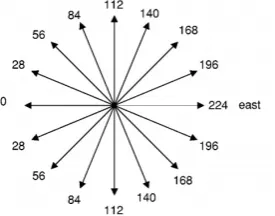
Quantisation:Based on [16], the magnitude and the direction of the mov-ing points are mapped into the Magnitude Plots and the Directional Plots. The magnitude is arbitrarily mapped into nine grey levels shown in Table 1. Regions of darker grey in the Magnitude Plots correspond to regions with larger normal flow magnitudes. The direction is mapped into nine grey levels as shown in Figure 1.

Figure 1: Quantisation of normal flow direction into 16 grey levels. (figure extracted from [16])

Extended Plots:The Extended Magnitude Plots (EMPs) and Extended Directional Plots (EDPs) [16] are calcu-lated in order to trace the motion history.τMagnitude Plots ft are "superimposed" to construct an EMP, where

t_∈[1,τ]is the position of the plot in the temporal domain. That is to say, the EMPF(i,j)at pixel locationi

andj takes the value of the last moving point in ft(i,j). It takes the value 255 iff1(i,j),f2(i,j),...,fτ(i,j)are

only stationary points. The EDPG(i,j)is similarly calculated fromτDirectional Plotsgt(i,j), resulting in 10 grey levels (9 directions and an extra level 255 for stationary points). Following the setup from [16], we choose

τ₌5.

Multiresolution:A basic multiresolution analysis is performed, with the purpose of demonstrating the potential of this approach in a DT classification problem. The original sequences are decomposed into several temporal resolutions by applying a Gaussian pyramid.

Dynamic Texture features:The co-occurrence matrices of the EMPs (9 by 9 matrices) and of the EDPs (10 by 10 matrices) are calculated and averaged over the whole sequence for each resolution. An angleθ₌0° and a distanced₌1pixel between the pixel neighbours are chosen in this experiment as a proof of concept. The final features are composed of the raw mean co-occurrence matrices of each resolution vectorized and concatenated in one single feature vector.

Rotation Invariance: In order to further estimate the robustness of the algorithm, rotation invariance is devel-oped in the feature extraction process. The rows and columns of the co-occurrence matrices are re-organised depending on the dominant orientation of the EDPs.This is similar to rotating the OF vectors so that the dom-inant direction always points leftwards. Hence, similar features are extracted, for instance, from sequences of cars moving in different directions.

Results and discussions The developed algorithm is tested on the Dyntex++ database [10]. It consists of 36

of the art in Table 3. The state of the art method which obtains the best results ([19]) uses PCA-cLBP (PCA on the concatenated LBP), PI-LBP (Patch-Independent), PD-LBP (Patch-Dependent) and a super histogram averaging the histograms across the sequence. Finally it uses a Radial Basis Function (RBF) SVM classifier. Our experiment does not aim to maximise the classification results, but rather to demonstrate the importance of the OF, the multiresolution analysis and the rotation invariance in a DT classification framework. It performs only 2.7%worse than the state of the art on the Dyntex++ database. The multiresolution analysis greatly improves the performance of our method from 74.8% to 89.7% with respectively one and four resolutions. Moreover, one could expect the classification success rate to dramatically drop with the rotation invariance since crucial information about the direction is lost. However, it is interesting to point out that we only measure a drop of 2.3%and 1.6%with respectively four and one resolutions.

number of resolutions 1 2 3 4

normal 74.8% 84.4% 87.4% 89.7%

rotation invariant 73.2% 82.5% 85.6% 87.4%

Table 2: Global classification results of our method on Dyntex ++ using one to four resolution images (starting from the original image and adding lower resolutions with the Gaussian pyramid).

Method Classification rate

DL-PEGASOS [10] 63.7%

Extended Plots - 4 resolutions (our method) 89.7%

PCA-cLBP/PI-LBP/PD-LBP+super histogram + RBF SVM [19] 92.4%

Table 3: Classification results comparison with the state of the art on Dyntex++.

Finally, it should be noted that some sequences are misclassified into classes with very similar motion. For instance, eight sequences of the class 27 "leaves on branches swaying with wind" are misclassified into the class 33 ("branches swaying in wind (no leaves)". Adding a spatial analysis to this method would overcome this issue.

4 Combined Co-occurrence Matrix of Optical Flow (CCMOF)

Introduction As shown in section 3, the co-occurrence matrix approach developed in [12, 13] can be used

to characterise the distribution of the OF. However, creating a co-occurrence matrix from a vector image is not as straightforward as the classic GLCM extracted from pixel intensities. Indeed, the occurrence of two values must be taken into account such as the x and y components of the flow vectors or their magnitudes and directions. This is why the EDPs and EMPs were used in [16]. However, analysing the two components separately gives rise to a loss of information carried by the joint distribution. Furthermore, the quantisation of the magnitude is not as simple as the quantisation of a grey-scale image or an orientation image. Grey-scale images and orientation images are respectively defined in the bounded intervals [0,255] and [-180,180], whereas the magnitude is only limited by the size of the image. In [16] and section 3, flow vectors with a magnitude larger than four pixels were considered as noise which is not the case in many DT sequences. Extending the quantisation to the maximum magnitude that a correct flow vector can have (maximum magnitude of all the sequences, up to 25 pixels length) is not a convenient solution either. In order to overcome these issues, a new framework combining the magnitude and the orientation of the flow is developed using individual quantisation levels of the magnitudes for each sequence.

Method description The framework of our CCMOF method is illustrated in Figure 2. The OF is calculated

Figure 2: Feature extraction diagram of the CCMOF.

resulting in 64 bins spanning the OF vector values. For each sequence, the magnitude is linearly quantized in eight bins in the ranges[0,Ms]([0,₈1Ms],[1₈Ms,2₈Ms],...,[7₈Ms,Ms]), whereMs is the largest magnitude of the sequence after removing large outliers which will not contribute to the CCMOFs, using Peirce’s criterion. Finally, the co-occurrence of the neighbouring flow vectors is calculated, resulting in three 64 by 64 CCMOFs; two for the spatial, one for the temporal domain. The matrices extracted in the space domain summarise the occurrence of the pairs of neighbours on the x and y axes. This co-occurrence is calculated on every frame, then summed over the entire sequence and normalised. In the time domain, the same process is applied with neighbours on the temporal axis. These co-occurrence matrices differ from the classic GLCM as they combine two dimensions. The definition of new features is necessary in order to extract the distributions of the magnitude and of the orientation as well as their joint distribution. In total, 19 features are calculated based on Haralick’s features [13]; 11 in the spatial domain and eight in the temporal domain: The Energy, Contrast,Orientation Contrast,Magnitude Contrast,Correlation,Sum of Squares,HomogeneityandEntropy are extracted from both the spatial and temporal CCMOFs. TheDominant Orientation,Dominant Magnitude andWeighted Dominant Orientation are calculated only in the spatial domain. We need to slightly modify the calculation of the Haralick’s features [13] regarding the difference n between neighbours. In Haralick’s features, the difference between neighbours n is defined as Equation (1) and represents the variation in the neighbours’ intensities.

n_{= |}i₋j_|, n_∈{q1,q2,...,qN}, (1) wherei,j_∈{q1,q2,...,qN} represent the quantised values of the pair of neighbours andq1,q2,...,qN are the

N discrete grey levels of quantization. In our case,n is chosen as the Manhattan distance between neighbour vectors (Equation (2)).

n_{= |}Mˆi−Mˆj| + |Oˆi−Oˆj| mod 4, n∈{0;1;2;...;11}, (2) where_Mˆ_{i, ˆMjare the quantised magnitudes of the neighbour vectors andO}ˆ_{i, ˆOj their orientations. On Figure 3,}

the distance between the two vectors isn₌2. Finally, it was observed that the smallest magnitudes in a vector image are often due to noise on a static part of the DT. For instance, in a traffic DT, OF vectors are calculated on the supposedly static road with magnitudes close to zero. Their orientation is therefore not relevant and reduces the discriminative power of the features calculated from the CCMOFs. Therefore, the same 19 features are calculated from the CCMOFs in which the bin corresponding to the smallest magnitudes is removed (resulting in 7 by 8 matrices). A total of 38 features is thus extracted from each DT sequence.

DT recognition, as proposed in [19], should largely rely on appearance analysis as it contains the most discrim-inative information. Therefore, we combine our motion features with LBP-TOP features [23]. Thus, we cover the analysis of the motion (CCMOF) in the spatiotemporal domain as well as the pixel intensities’ distribution (LBP-TOP) in the spatiotemporal domain.

Results and discussion A sequential feature selection is applied in order to determine those which

Figure 3: OF quantisation with two vector examples (_Mˆ _{= 7,O}ˆ _{= 6 (left);M}ˆ _{= 6,O}ˆ _{= 7 (right)).}

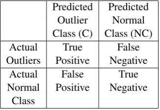
We sought to rectify those by focusing on videos which exhibit only one DT and contain the same dynamic on the entire space-time domain. We also select sequences which depict different scenes, from various viewpoints. The resulting dataset contains 10 classes of DTs, each with 20 sequences of size 100*100*50. The experi-mental setup is the same as in section 3. 10 sequences are randomly selected from each class for the training set. The other 10 sequences are used for testing. The confusion matrix presenting the classification results using the CCMOF features in combination with LBP-TOP is shown in Figure 4 and the overall classification results are presented in Table 4. One can notice that the main misclassifications occur for very similar classes ("water"/"waves" and "foliage"/"trees") which share similar dynamics and spatial texture.

Figure 4: Confusion matrix of CCMOF + LBP-TOP on the developed database.

Method Classification rate

CCMOF 68.0%

LBP-TOP [23] 81.7%

LBP-TOP + CCMOF 84.4%

Table 4: Classification results of CCMOF and LBP-TOP on the developed database.

The motion analysis using the CCMOF approach significantly improves the classification of our dataset when combined with the analysis of the spatiotemporal distribution of the pixel intensities (LBP-TOP). Solely analysing the motion is not sufficient to obtain a classification as accurate as the literature. It confirms that a DT recogni-tion system mostly relies on the spatial texture analysis [19] and the morecogni-tion analysis provides complementary information that can improve the performance.

5 Conclusion

References

[1] E. H. Adelson and J. R. Bergen. Spatiotemporal energy models for the perception of motion. JOSA A, 2:284–299, 1985.

[2] T. Boujiha, J.-G. Postaire, A. Sbihi, and A. Mouradi. New approach for dynamic textures discrimination. pages 1–4, 2010.

[3] C.-C. Chang and C.-J. Lin. Libsvm: a library for support vector machines. ACM Transactions on Intelli-gent Systems and Technology (TIST), 2:27, 2011.

[4] J. Chen, G. Zhao, M. Salo, E. Rahtu, and M. Pietikainen. Automatic dynamic texture segmentation using local descriptors and optical flow. Image Processing, IEEE Transactions on, 22:326–339, 2013.

[5] K. G. Derpanis and R. P. Wildes. Dynamic texture recognition based on distributions of spacetime oriented structure. pages 191–198, 2010.

[6] G. Doretto, A. Chiuso, Y. N. Wu, and S. Soatto. Dynamic textures. International Journal of Computer Vision, 51:91–109, 2003.

[7] S. Fazekas and D. Chetverikov. Dynamic texture recognition using optical flow features and temporal periodicity. pages 25–32, 2007.

[8] A. B. Flores, L. A. Robles, R. M. M. Tepalt, and J. D. C. Aragon. Identifying precursory cancer lesions using temporal texture analysis. pages 34–39, 2005.

[9] P. Gao and C. L. Xu. Extended statistical landscape features for dynamic texture recognition. volume 4, pages 548–551, 2008.

[10] B. Ghanem and N. Ahuja. Maximum margin distance learning for dynamic texture recognition. pages 223–236. 2010.

[11] W. N. Gonçalves, B. B. Machado, and O. M. Bruno. Spatiotemporal gabor filters: a new method for dynamic texture recognition. arXiv preprint arXiv:1201.3612, 2012.

[12] R. M. Haralick. Statistical and structural approaches to texture. Proceedings of the IEEE, 67:786–804, 1979.

[13] R. M. Haralick, K. Shanmugam, and I. H. Dinstein. Textural features for image classification. Systems, Man and Cybernetics, IEEE Transactions on, pages 610–621, 1973.

[14] Y. Hu, J. Carmona, and R. F. Murphy. Application of temporal texture features to automated analysis of protein subcellular locations in time series fluorescence microscope images. pages 1028–1031, 2006. [15] Z. Lu, W. Xie, J. Pei, and J. Huang. Dynamic texture recognition by spatio-temporal multiresolution

histograms. volume 2, pages 241–246, 2005.

[16] C.-H. Peh and L.-F. Cheong. Synergizing spatial and temporal texture.Image Processing, IEEE Transac-tions on, 11:1179–1191, 2002.

[17] Y.-l. Qiao and F.-s. Wang. Dynamic texture classification based on dual-tree complex wavelet transform. pages 823–826, 2011.

[19] J. Ren, X. Jiang, and J. Yuan. Dynamic texture recognition using enhanced lbp features. pages 2400–2404, 2013.

[20] P. Saisan, G. Doretto, Y. N. Wu, and S. Soatto. Dynamic texture recognition. volume 2, pages II–58, 2001.

[21] L. C. Sincich and J. C. Horton. The circuitry of v1 and v2: integration of color, form, and motion. Annu. Rev. Neurosci., 28:303–326, 2005.

[22] D. Sun, S. Roth, and M. J. Black. Secrets of optical flow estimation and their principles. pages 2432–2439, 2010.

[23] G. Zhao and M. Pietikainen. Dynamic texture recognition using local binary patterns with an application to facial expressions. Pattern Analysis and Machine Intelligence, IEEE Transactions on, 29:915–928, 2007.

Investigation into DCT Feature Selection for Visual Lip-Based

Biometric Authentication

C Wright, D Stewart, P Miller, F Campbell-West

Centre for Secure Information Technologies (CSIT) Queen‘s University Belfast

{cmclarnon03, Dw.Stewart, p.miller, f.h.campbellwest} @qub.ac.uk

Abstract

This paper investigated using lip movements as a behavioural biometric for person authentication. The system was trained, evaluated and tested using the XM2VTS dataset, following the Lausanne Protocol configuration II. Features were selected from the DCT coefficients of the greyscale lip image. This paper investigated the number of DCT coefficients selected, the selection process, and static and dynamic feature combinations. Using a Gaussian Mixture Model - Universal Background Model framework an Equal Error Rate of 2.20% was achieved during evaluation and on an unseen test set a False Acceptance Rate of 1.7% and False Rejection Rate of 3.0% was achieved. This compares favourably with face authentication results on the same dataset whilst not being susceptible to spoofing attacks.

Keywords:Authentication, Biometrics, GMM-UBM, XM2VTS, DCT

1 Introduction

It is widely recognised that passwords are not enough to use as a sole means of authentication, which has been made apparent by many high profile hacking cases. This has resulted in biometric authentication becoming increasingly popular. Physiological-based biometric systems have been incorporated into the most common mobile platforms, i.e. Android’s Face unlock and iPhones fingerprint scanner, and have been hacked using replay attacks and spoofing [Racoma, 2012], [Kleinman, 2014]. Behavioural biometrics are potentially more difficult to crack but are also more complex to capture, model and authenticate robustly.

In this area ’Speaker Verification’ is acknowledged as the ability to authenticate a person’s claimed identity from their voice [Campbell, 1997]. Gaussian Mixture Model–Universal Background (GMM-UBM) systems are commonly used with speaker verification systems, [Hautamäki et al., 2015]. The set up involves using creating a GMM to model each individual, and another large GMM that represents the whole population – the UBM. When authenticating a person’s claimed identity, a likelihood is calculated with respect to their individual model and another with respect to the UBM. A resulting score can be calculated using these likelihoods.

[Cetingul et al., 2006] researched lip motion features for speaker and speech recognition using Hidden Markov Models (HMMs). Features evaluated include dense motion features within a bounding box around the lips, and features created from lip shape (contours) and motion. The MVGL-AVD database consisting of 50 individuals was used. The best recorded result for speaker recognition was found during the cross validation of the system using motion features with an Equal Error Rate (EER) of 5.2%.

[Faraj and Bigun, 2006] investigated a combination of audio and visual features from the lips for person authentication. Experiments used Gaussian Mixture Models (GMM), the XM2VTS database and the Lausanne Protocol, configuration I. Results reported an EER of 22% on visual features alone.

Protocol, configuration II was followed [Luettin and Maître, 1998] in an attempt to rigorously benchmark this system and allow for comparison. Discrete Cosine Transform (DCT) coefficients of greyscale lip images were used as visual lip features. As with existing speaker verification systems a likelihood value was calculated using both models of the claimed individual and the UBM.

2 DCT Features

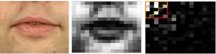
Figure 1: Individual 0, Session 1, video 1, frame 1. From left to right: Pre-processed cropped image, Grey scale resized image, DCT coefficients of the frame with both square and triangular mask

The DCT coefficients were chosen as they can cap-ture lip appearance in a compact form. Investigating gender recognition [Stewart et al., 2013] used DCT coefficients as a feature, the positive results demon-strate that they captured speaker specific appearance and dynamics. However there has been no rigorous investigation of DCT-based features for speaker au-thentication which is the aim of this work.

Although we are aware that DCT coefficients can be useful for modelling lip appearance, we do not

know how many DCT coefficients are required to effectively model identities and we do not know the rela-tive utility of static DCT coefficients compared to their derivarela-tive features. Furthermore when extracting DCT coefficients as features from the full DCT coefficient matrix, two common masks can be applied, square or triangular. It has been shown for lip-based speech recognition that a triangular mask offers better performance, [Stewart et al., 2013], and we will seek to establish if the same is true when modelling identities.

Figure 1 shows how the video data is processed during these experiments. The first image shows the cropped Region Of Interest (ROI). Next each frame is converted to grey scale. After histogram equalisation the frame is resized to a 16 by 16 pixel image, this is shown in the second image in figure 1. The third image shows a visual representation of the 2D DCT coefficients of the frame overlaid with both square and triangular masks. The masks were used to extract the required number of DCT coefficients,k. The extracted DCT coefficients of the jthframe are represented byxj, ak£1column vector. The frames are stacked to make ak£n matrix, where n is the number of frames in a video,X={x1,x2,...,xn}. Normalisation was used to reduce the effects of inter-session variability using:

xi_j=(x

i j°µi)

æi , (1)

whereµi is the mean of theith DCT coefficient across all frames, similarly æi is the standard deviation.

The resulting normalised feature for the entire video input is therefore:X={x1,x2, ...,xn}.The same steps were used to prepare the videos for all steps in the training, evaluation and testing.

3 GMM Modelling

GMMs were used to represent both the UBM and the individual models. During an attempted login the system will test the input against the claimed individual model and against the UBM. UsingX, we want to compute how alike it is to the features that created a model,∏. The likelihoodp(X|∏), is calculated using:

p(X|∏)=

n Y

j=1 M X

i=1

!i pi°x, j¢ (2)

pi°xj¢= 1

(2º)k2|_ßi|12

exp

Ω

°1₂°xj°µi¢T(ßi)°1°xj°µi¢ æ

(3)

4 Classification

We want to compute the likelihood that the feature extracted from the video input, X, was generated by the claimed identity, and the likelihood that the feature was not generated by the claimed identity. If we denote the likelihood ofXbeing generated by the claimed identity as p(X|∏hyp),where ∏hyp represents the mean vector and covariance matrix parameters of the hypothesised Gaussian model, and the likelihood ofXof being generated by anybody else as p(X|∏U B M), where ∏U B M represents the mean vector and covariance matrix parameters of the UBM Gaussian model. Then a log-likelihood ratio can be calculated using equation 4:

§(X)₌log p(X|∏hyp)°logp(X|∏U B M) (4) The log-likelihood generated from equation 4 can then be tested against the threshold and the identity accepted or rejected as shown in the modular diagram in figure 2.

5 Experiments

The aim of these experiments was to investigate the feature representation that produced the lowest EER when varying:

• The mask type used to select the number of DCT coefficients. The right most image in figure 1 shows both triangular and square masks.

• The number of DCT coefficients. Square masks were tested from a 3 by 3 mask producing a feature vector containing 9 DCT coefficients to a 7 by 7 mask producing 49 DCT coefficients. For the triangular masks the range went from a 4 by 4 mask producing 10 DCT coefficients to a 9 by 9 mask producing 45 DCT coefficients.

• The ’type’ of feature, ie. Static / Dynamic. This work looked into the performance of static, dynamic and combinations of both to help find the optimum feature representation.

The dynamic features included the first and second order derivatives of the static DCT coefficients with respect to time, known as delta, ¢, and deltadelta, ¢¢, features. After testing the features separately, all combinations of the 3 features were tested. The features are combined by concatenating the feature vectors. For example if 15 DCT coefficients had been selected, when combining static and¢, the¢¢, DCT coefficients were concatenated after the static making a total of 30 DCT coefficients.

5.1 System Overview

Figure 2: General Modular Diagram of the System Figure 2 shows a modular diagram showing how the

system was used during testing. After a video was read in the features were extracted and normalised as described in section 2. The features are used to get a log-likelihood from the claimed GMM and the UBM as described in section 3, and a log-likelihood ratio was obtained using equation 4. The ratio log-likelihood will be either accepted or rejected based

5.2 Database and Protocol

Experiments were carried out on the XM2VTS [Messer et al., 1999]. The XM2VTS is a large audio-visual database containing video recordings of 295 individuals during 4 sessions. Each session contains 2 videos per person and the sessions were recorded over 4 months. For these experiments only digit sequences spoken during recording sessions were used. Pre-processed video data was also used as the audio was removed and the video was cropped to only contain mouth region, for preprocessing steps see [Seymour et al., 2008].

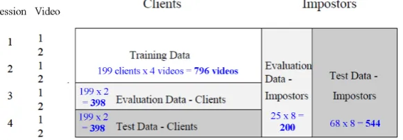
For these experiments the Lausanne Protocol [Luettin and Maître, 1998], configuration II was strictly fol-lowed. The Lausanne Protocol is a closed-set verification protocol [Bourlai et al., 2005], because the population of clients does not change the system does not need to account for new users in the evaluation and testing. As shown in figure 3, the protocol divides the dataset into Training, Evaluation and Test data.

• The Training data consists of video from the first 2 sessions for 200 individuals.

• The Evaluation data consists of video data from the third session for the same 200 individuals. Plus all video data for a separate 25 individuals not used in training. See section 5.4 for more details on how these videos are used to represent returning clients and imposters.

• The Test data is made up of the 2 videos from the fourth session of the 200 individuals used for training, plus all video data available for a separate 70 individuals not used in the training.

Data from 3 individuals was removed from our tests as some vidos were found to be corrupt. The IDs of the individuals removed are 342, 272 and 313. Figure 3 shows the number of individuals used in these experiments after the corrupt videos were removed.

Figure 3: Partitioning of the XM2VTS database according to the protocol Configuration II 5.3 Training

The UBM was trained with all the designated Training data as specified in figure 3, 796 videos from 4 individ-uals. General guidelines for unconstrained speech suggest 512-2048 Mixtures for the UBM, where lower-order mixtures are more common with constrained speech such as digits and fixed vocabulary [Bimbot et al., 2004]. For the experiments in this work all UBMs were trained with 256 mixtures as all video data contains dig-its. Individual GMMs were created for each of the 199 individuals in the training data and each model was created using 32 mixtures, likewise 32 mixtures has been used in speaker recognition for individual models, [Stewart et al., 2013].

5.4 Evaluation

Evaluation was carried out in order to select a threshold before running the system on the unseen Test data, using the Evaluation data specified in figure 3. All 598 videos were tested against all 199 individual models, producing

Figure 4: Evaluation results for Static,¢,¢¢features.

The graphs in figure 4 show the EER against the number of DCT coefficients. The graphs show the static, ¢and¢¢features. It can be seen that the triangular feature selection outperforms the square feature selection. All 3 graphs show that as the number of DCT coefficients increases the EER is reduced, and it appears that no additional information is gained by using more than 28 DCT coefficients. It can also be seen that the Static features produce the highest EER, and the¢features produced the lowest EER.

No. DCT coefficients

Features 15 21 28 36

Static 5.28 4.34 4.73 3.91

¢ 2.59 2.63 2.20 2.51

¢¢ 3.25 3.09 3.14 3.02

Static &¢ 3.59 3.27 3.27 3.52 Static &¢¢ 4.02 3.98 4.02 3.52 ¢&¢¢ 3.10 3.52 2.94 3.27 Static,¢&¢¢ 3.02 3.69 3.52 3.94

Table 1: Equal Error Rate (%) on Evaluation set: Showing highest performing number of DCT coefficients, selected used a triangular mask.

Following this, experiments were then run to test combinations of static,¢and¢¢features using triangular feature selection and 15, 21, 28 and 36 DCT coefficients. Combining the static and dynamic information did not appear to add additional information to the features as the¢alone produced the lowest EER, 2.20%. Results can be seen in table 1.

5.5 Testing

From the evaluation, the set up producing the lowest EER was found to be triangular features using 28¢DCT coefficients. The optimum threshold for this system was then calculated based on the EER and applied for testing the unseen data. Before running the unseen Test data on the system using the threshold calculated, practice dictates that the system is retrained using both the Training and Evaluation data [Hastie et al., 2009]. These experiments investigated both this practice and running the unseen Test data on the system without retraining. In theory a system would be trained with all available data before deployment and a threshold calculated based on the data it was trained on. If we retrain the models with the Evaluation data it would be expected the threshold calculated in the evaluation would no longer be optimum therefore the unseen data would be expected to not perform as well.

The 942 videos were tested against all the 199 individual models. This produced 942£199=187,458

FRR FAR Models Not Retrained 3.02% 1.68% Models Retrained 1.76% 4.21%

Table 2: False Rejection Rate (FRR) & False Acceptance Rate (FAR) for unseen test data.

Note the performance (in terms of both FAR and FRR) from evaluation for these same models with the same operating threshold was 2.20%. As seen in table 2, a FRR of 3.02% and FAR of 1.67% was obtained.

On the bottom row of table 2 we can see the results for the Test data after evaluation, when the models have been retrained to contain all the Training and Evaluation data. The table shows a FRR of 1.76% and a FAR of 4.21%.

Figure 5: Histogram showing the Client & Imposter Log Likelihoods. Left to right: Not retrained, Retrained The image on the left in figure 5 shows a histogram of the normalised log-likelihoods of the Test data and the threshold is marked on with a dashed line. There is small overlap in clients and imposters around the threshold. We can see that no matter what threshold was chosen in this experimental setup there will always be FAR or FRR, but the chosen threshold does appear to minimise both the FAR and FRR for unseen data. The image on the right in the figure shows the normalised log-likelihoods for the retrained setup. By comparing the histograms in figure 5 we can see how the threshold set for models trained with less data is no longer optimum with increased training data. This means that if the model is retrained with more data a new threshold should be calculated as in the evaluation stage of these experiments. The overlap of imposters and clients also appears to have reduced in this histogram, indicating that the system improves with more Training data.

As the threshold was set during evaluation, the top row in table 2 shows the true results on unseen data after training and evaluation. These results show even with limited Training data the system successfully authenticated 96.98% of registered clients and successfully prevented access to 98.32% of the imposters.

These results compare very favourably with previous lip based authentication results even though some were on much smaller datasets, [Cetingul et al., 2006]. On the Evaluation data we achieved an EER of 2.2%, producing a predicted performance of 97.8%. This is an improvement on [Cetingul et al., 2006] et al who recorded an error rate of 5.2%. Faraj et al [Faraj and Bigun, 2006] recorded a performance of 78% for the visual features on their own. The EER was used to calculate a threshold which was used to test unseen Test data, this gives a more accurate result on how the system would work in a deployment scenario. These tests produced a FAR of 1.7% and a FRR of 3.0%.

The DCT-based features compare well with results recorded in [Bhattacharjee and Sarmah, 2012], where a 4.55% EER was achieved with a GMM-UBM system and audio features for authentication.

and on the Test set a FAR and FRR of 1.35% and 0.75% respectively.

Upon further analysis of the specific test cases which caused the FRR errors to occur. The 3.02% of FRR errors equated to 12 attempted logins from only 9 individuals from the 199 registered individuals in the system. Of these, only 3 individuals failed to be authenticated as themselves on both of their test videos. Therefore only 1.5% of individuals could not be authenticated successfully if at least two attempts were considered.

Figure 6 illustrates the data for the 3 problematic individuals. Upon close inspection, the most obvious reason for individual 79 not being authenticated appears to be inconsistent registration of the lip ROI which led to slight rotation of the Test dataset frames compared to the Training frames. Similarly, it is inconsistent ROI extraction which appears to have caused the error for individual 264. In this case the individuals facial hair may have caused the poor lip tracking. For individual 191 the error appears to be caused by a significant change in facial hair prior to the test.

Figure 6: From top down, individual 79, 191, 264. From left to right: Frames 1-4 are from each video included in model, Frames 5-6 are from each video that failed to login

6 Conclusion

This work provided a rigorous investigation of the effectiveness of DCT-based features for modelling speaker’s lips within a GMM-UBM verification framework. In particular, we investigated the performance of different numbers of DCT coefficients, different selection of masks and different DCT-based feature types. The types included the static DCT coefficients and their first and second order derivatives known as¢and¢¢ features. The largest available dataset for such experiments was used, including 292 individuals, namely the XM2VTS database along with the robust Lausanne Protocol configuration II. We showed for the first time that:

• ¢features produced the best feature representation over static,¢¢and multiple combinations • 28 DCT coefficients were found to be optimal for the feature

• Triangular mask used in feature selection is better than a square mask

On the Evaluation set an EER of 2.2% was obtained, producing a predicted performance of 97.8%. The EER was used to calculate a threshold which was used to test unseen data, this gives amore accurate result on how the system would work in a deployment scenario. These tests produced a FAR of 1.7% and a FRR of 3.0%. These results compare very favourably with previous works in verification and authentication using alter-native features and models, and compared to facial recognition systems using the same database and protocol.

Our analysis of the errors indicates that the system performance can be affected by poor and inconsistent lip ROI tracking. We will be investigating this further in our future work.

References

[Bimbot et al., 2004] Bimbot, F., Bonastre, J.-F., Fredouille, C., Gravier, G., Magrin-Chagnolleau, I., Meignier, S., Merlin, T., Ortega-García, J., Petrovska-Delacrétaz, D., and Reynolds, D. A. (2004). A tutorial on text-independent speaker verification. EURASIP J. Appl. Signal Process., 2004:430–451.

[Bourlai et al., 2005] Bourlai, T., Messer, K., and Kittler, J. (2005). Scenario based performance optimisation in face verification using smart cards. InAudio-and Video-Based Biometric Person Authentication, pages 289–300. Springer.

[Brady et al., 2007] Brady, K., Brandstein, M., Quatieri, T., and Dunn, B. (2007). An evaluation of audio-visual person recognition on the xm2vts corpus using the lausanne protocols. In Acoustics, Speech and Signal Processing, 2007. ICASSP 2007. IEEE International Conference on, volume 4, pages IV–237. IEEE. [Campbell, 1997] Campbell, J.P., J. (1997). Speaker recognition: a tutorial. Proceedings of the IEEE,

85(9):1437–1462.

[Cetingul et al., 2006] Cetingul, H. E., Yemez, Y., Erzin, E., and Tekalp, A. M. (2006). Discriminative analysis of lip motion features for speaker identification and speech-reading. Trans. Img. Proc., 15(10):2879–2891. [Faraj and Bigun, 2006] Faraj, M. and Bigun, J. (2006). Motion features from lip movement for person

au-thentication. InPattern Recognition, 2006. ICPR 2006. 18th International Conference on, volume 3, pages 1059–1062.

[Hastie et al., 2009] Hastie, T. J., Tibshirani, R. J., and Friedman, J. H. (2009). The elements of statistical learning : data mining, inference, and prediction. Springer series in statistics. Springer, New York. Autres impressions : 2011 (corr.), 2013 (7e corr.).

[Hautamäki et al., 2015] Hautamäki, R. G., Kinnunen, T., Hautamäki, V., and Laukkanenn, A.-M. (2015). Automatic versus human speaker verification: The case of voice mimicry.Speech Communication.

[Kleinman, 2014] Kleinman, Z. (2014). Politician’s fingerprint ’cloned from photos’ by hacker. http://www.bbc.co.uk/news/technology-30623611.

[Luettin and Maître, 1998] Luettin, J. and Maître, G. (1998). Evaluation protocol for the extended M2VTS database (XM2VTSDB). Idiap-Com Idiap-Com-05-1998, IDIAP.

[Messer et al., 2003] Messer, K., Kittler, J., Sadeghi, M., Marcel, S., Marcel, C., Bengio, S., Cardinaux, F., Sanderson, C., Czyz, J., Vandendorpe, L., Srisuk, S., Petrou, M., Kurutach, W., Kadyrov, A., Paredes, R., Kadyrov, E., Kepenekci, B., Tek, F., Akar, G. B., Mavity, N., and Deravi, F. (2003). Face verification compe-tition on the xm2vts database. InIn 4th Int. Conf. Audio and Video Based Biometric Person Authentication, pages 964–974.

[Messer et al., 1999] Messer, K., Matas, J., Kittler, J., and Jonsson, K. (1999). Xm2vtsdb: The extended m2vts database. InIn Second International Conference on Audio and Video-based Biometric Person Authentica-tion, pages 72–77.

[Murphy, 2001] Murphy, K. P. (2001). The bayes net toolbox for matlab. InComputing Science and Statistics. [Racoma, 2012] Racoma, J. A. (2012). Android jelly bean face unlock ’liveness’ check easily hacked with

photo editing. http://www.androidauthority.com/android-jelly-bean-face-unlock-blink-hacking-105556. [Seymour et al., 2008] Seymour, R., Stewart, D., and Ming, J. (2008). Comparison of image transform-based

features for visual speech recognition in clean and corrupted videos. J. Image Video Process., 2008:14:1– 14:9.

3D Reconstruction of Reflective Spherical Surfaces from Multiple

Images

Abdullah Bulbul, Mairead Grogan & Rozenn Dahyot

School of Computer Science and Statistics Trinity College Dublin, Ireland {bulbulm, mgrogan, Rozenn.Dahyot}@tcd.ie

Abstract

Despite the recent advances in 3D reconstruction from images, the state of the art methods fail to ac-curately reconstruct objects with reflective materials. The underlying reason for this inaccuracy is that the detected image features belong to the reflected scene instead of the reconstructed object and do not lie on the surface of the object. In this study, we propose a method to refine the 3D reconstruction of reflective convex surfaces. This method utilizes the geometrical distortion of the reflected scenes behind a spherical surface.

Keywords:3D reconstruction, Shape from images, Hough Transform, Specular surface

1 Introduction

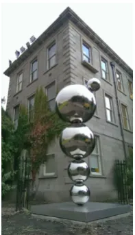
Figure 1: Walton Sculpture (Trinity college Dublin Ireland).

Creating 3D worlds in the form of meshes that can be efficiently manipulated by engines has found many applications from com-puter games and virtual reality, to virtual museums visits. To assist artists in the creation of 3D meshes of real existing ob-jects, many software systems have been developed using RGB or RGB-D images and videos.

In this paper we have created a dataset of images captured around a sculpture made of specular material, which is com-posed of several spherical elements (cf. Fig. 1). Using this dataset we propose to infer a 3D model of the sculpture by us-ing several image processus-ing routines. First a 3D point cloud is computed using the set of images. Each element of this point cloud has vertex, colour RGB and normal information. From this information we propose a Hough Transform like process to infer the centers and radii of the spheres. Such compact information allows us to easily generate a 3D representation convenient to use in a virtual environment such as Metropo-lis [O’Sullivan, 2010].

2 State of the Art

2.1 3D reconstruction

system does to perceive the world in 3D using triangulation based depth cues, e.g, stereo vision, motion paral-lax. In computer graphics and vision literature this procedure is called Structure from Motion (SfM). An earlier complete model of 3D reconstruction from unordered photos is given by Pollefeys et al. [Pollefeys et al., 2004]. In a well known study, Snavely et al. [Snavely et al., 2006] proposes a sparse 3D reconstruction method and im-proves the methods proposed in [Brown and Lowe, 2005] and [Hartley and Zisserman, 2004]. Using the sparse reconstruction output, Furukawa and Ponce generate dense 3D point clouds [Furukawa and Ponce, 2010]. An-other similar study utilizes sparse 3D reconstructions to generate separate depth maps for each input image [Goesele et al., 2007]. Then these depth maps are used for dense 3D reconstruction.

Recently SfM studies have advanced in terms of the employed parallelism [Agarwal et al., 2011], perfor-mance [Frahm et al., 2010, Wu, 2013], which enables using a high number of input images, and symmetry de-tection [Cohen et al., 2012, Ceylan et al., 2014] which improves the accuracy of the outputs. All of these stud-ies rely on corresponding feature matches among multiple images to determine a point in the 3D environment. However, for reflective surfaces these correspondences do not reside exactly on the surface of an object, which causes incorrect 3D reconstructions around the reflective surfaces. In order to refine reconstruction of scenes in-cluding planar reflective surfaces, Wanner and Goldluecke [Wanner and Goldluecke, 2013] propose a method that uses images from a regular structure of viewpoints. Another group of studies that work on reconstruc-tion of reflective objects uses specular flow informareconstruc-tion [Roth and Black, 2006, Sankaranarayanan et al., 2010, Balzer et al., 2011]. In these studies, reflected objects are known and the way they are distorted is utilized for estimating surface geometry. In our case, neither the viewpoints are distributed regularly nor the reflected objects are known; therefore, none of these studies are directly applicable.

2.2 Sphere detection in point clouds

The Hough Transform is a standard popular technique for finding parametric shapes. It is a one-to-many map-ping approach where each observation votes for multiple models (e.g. lines). This corresponds to computing a histogram in the latent space of the parameters describing the shape, and the bins collecting the most votes are deemed as potential candidate occurrences of the shape of interest. This technique can be difficult to use when dealing with noisy data and for exploring high dimensional latent spaces. To find spheres in 3D images, Cao et al have proposed a hierarchical Hough transform based technique by first finding circles in 2D image slices [Cao et al., 2006]. A sphere is then inferred by correlating circle parameters.

To alleviate the discrete histogram formulation of the Hough Transform, Dahyot proposed smooth kernel density estimates (KDE) to aggregate all votes for finding lines [Dahyot, 2009]. Moreover, when normal infor-mation extracted from gradient direction inforinfor-mation of images is available, it can also easily be encapsulated in the KDE. However no extension of this KDE modeling to circle or sphere is available yet.

Schnabel et al. [Schnabel et al., 2007] proposed a many-to-one RANSAC based technique for finding multi-ple shapes (plane, sphere, cylinder, cone, torus) in 3D point clouds containing vertices augmented with normals. RANSAC is not designed to detect multiple occurrences of a shape and this limitation is overcome by using localised sampling. We propose here a global Hough based approach for finding multiple spheres occurring in noisy point clouds (vertices and normals) computed from images.

3 Geometry of Reflections in a Convex Surface

p

c1 c2

c3 p'₂₃

p'₁₂ p'₁₃

p'₂₃

p'₁₂ p'₁₃

(a) (b)

Figure 2: (a) Pairwise matchesp0

i,j of a reflected pointp among 3 different views. (b) Distortion of reflected shape and normals. Reflection of a straight feature is curved behind the spherical surface and the normal lines of the reflection converge.

Despite the lack of a stable reflection location, pairwise matches among viewpoints result in 3D reconstruc-tions of the reflected geometry inside the sphere as shown in Figure 3. Having a pair of viewpoints, similarly with stereoscopic vision, reflections of a scene over a spherical surface appear behind the surface of a sphere and the geometry is curved (Figure 2-b ). The generated vertices are distributed between the sphere surface and its focal distance (r/2) according to the actual distances of the reflected points.

(a) (b)

Figure 3: (a) A slice of the reconstructed point cloud belonging to the spherical surface shown on the left. (b) The same point cloud with per-vertex normals. Point clouds are generated by visualSFM [Wu, 2013] and the dense reconstruction method of [Furukawa and Ponce, 2010].

4 3D reconstruction from images

Figure 4: Overview of the proposed 3D reconstruction method. 4.1 Computation of the 3D point cloud

The proposed method works with an unordered set of images taken with a handheld camera or using the im-ages from photo-sharing websites and social media. An SfM based method is used to generate a sparse 3D reconstruction using SIFT feature matches. There are several methods for sparse reconstruction and bundle adjustment such as the ones proposed by [Snavely et al., 2006, Lourakis and Argyros, 2009]. We have used the sparse reconstruction implementation in VisualSFM [Wu, 2013], which is a publicly available tool for 3D reconstruction.

Similarly, dense 3D reconstructions could be obtained by employing the methods of [Furukawa and Ponce, 2010] or [Goesele et al., 2007]. Both of them gave high quality dense reconstructions in our trials and we have used Furukawa and Ponce’s method. The resulting sparse and dense reconstructions can be seen in Figure 5.

(a) (b) (c)

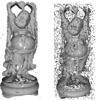
Figure 5: (a) One of the 122 input images, (b) sparse reconstruction, (c) dense reconstruction

4.2 Extracting Spheres Using Normal Correspondances

Figure 6: Intersection of two rays.

As explained in Section 3, per-vertex normals of a reconstructed spherical region with a reflective surface have a high probability of intersecting at locations inside the corresponding sphere. Therefore, we employ a special type of Hough Transform to determine these intersection points.

Finding candidates.AssumingV is the set of all vertices in the point cloud,

rays is calculated as follows:

di,j= ¯ ¯ ¯

¯(vi−vj).

ni×nj

kni×njk ¯ ¯ ¯

¯. (1)

Another key property of a valid intersection pointipis that the distances betweenipand the related vertices

should be approximately the same, as indicated in Figure 2-b. Lastly, in order to avoid classifying very close and parallel vertices, which are very common in dense reconstruction of planar surfaces, as valid intersection points; a third rule is set. This rule enforces the valid line pairs to get closer to each other towards the intersection point. Simply, the following equation must hold:

kvi−vjk >k ², (2) wherekis a parameter greater than 1 that adjusts the firmness of this rule. As we know that a valid intersection point hasdi,j<², this rule ensures that we avoid parallel lines. A lowerkvalue results in more candidate points and decreases performance, while a high value causes eliminating good candidates. We have empirically setk

to 16. Combining these three rules, we define the set of all valid intersection points (I P) as follows:

I P₌

(

(vi,vj)∈V,ip_i,j|¡di,j<²¢∧¡kvi−vjk >k ²¢∧ Ã

0.9_<kvi−ipi,jk

kvj−ip_i,jk<1.1

!)

. (3)

Voting procedure.After determining the candidate points, a voting procedure is performed with them. For that

purpose, each line defined byviandni votes for a candidate point inI Pif it passes through its²proximity. The intersection points with the most votes are selected as the valid candidate centers. The median of the distances between an intersection point and all of its voters is assigned as the radiusr(ip)of this intersection point ip

to be used in later steps. Figure 7 shows the set of intersection points and the selected intersections after the applied Hough Transform.

(a) (b) (c)

Figure 7: (a) Initial dense point cloud. (b) Candidate intersection points,I P. (c) Selected intersections after the voting procedure.

Merging close intersection points. As shown in Figures 2 and 3, there are multiple intersection points inside

of a sphere due to the specular nature of the sphere’s material. Normals belonging to different reflected objects intersect at different positions. Therefore, these intersection points are merged to get the final sphere locations. Two intersection points are merged if either of the intersection points lie inside the sphere formed by the other intersection point and its radius. When merging two intersection points ip_i andip_j ∈I P, properties of the

merged intersection pointip_m are assigned as follows.

    

ip_m =wi ip_i+wj ip_j,

r(ip_m) =wi r(ip_i)+wjr(ip_j)

V(ip_m) =V(ip_i)∪V(ip_j)

whereV(ip)is the set of vertices which voted foripandwi andwj are the weights assigned proportional to the sizes ofV(ip_i)andV(ip_j)respectively. All selected intersection points conforming to the merging criteria are

successively merged resulting in the final set of spheres (See Figure 8-b).

(a) (b) (c)

Figure 8: (a) Selected intersections before merging, (b) Final intersection points, used as the sphere centers. (c) Spheres with estimated radii.

vertex num (normalized between 0-100)

0 20 40 60 80 100

D ist a n ce t o ce n te r 0 0.5 1 1.5 2 2.5 3

3.5 Distribution of vertex-center distances

sphere 1 (smallest) sphere 2 sphere 3 sphere 4 (largest)

Figure 9: Each line corresponds to a different sphere.

Estimating the radius. Figure 9 shows the distribution of

distances between a sphere center and the vertices belong-ing to the correspondbelong-ing spheres. Except for some outliers, all of the vertices are expected to reside inside the sphere or over its surface. Therefore, after eliminating the outliers, determining the largest of the distances between a sphere center and corresponding vertices gives a reliable radius es-timation. As seen from Figure 9, the sorted distance curves change smoothly up to a point that indicates the presence of outliers. Assume thatD is the descendingly sorted dis-tances (outliers come first) andD0_{is its rate of change. The} first distanced∈Dwithd0<2∗mean(D0)is selected as the radius. The resulting spheres are illustrated in Figure 8-c.

Refining point cloud.After detecting the spheres, all

ver-tices inside the spheres are projected onto the sphere sur-face using the following formula.

v0₌v₊ r(ip)(v−ip)

kv₋ipk, (5)

where v0 _{is the updated location of vertex v inside a sphere with center ip and radius r(ip). The resulting} positions could be kept as a point cloud or could be used for surface reconstruction. Figure 10 shows the reconstructed surface using our method and presents its effectiveness.

5 Conclusion

Figure 10: Comparison with the state of the art pipeline (left) using VisualSFM [Wu, 2013] for point cloud generation followed by Poisson Surface Reconstruction [Kazhdan et al., 2006]. On the right, the result of our reconstruction by adding our reflective spherical surface refinement step after point cloud generation.

recreate a more realistic 3D model using images captured from multiple sources (e.g. social media images or drone footage).

Acknowledgments

This work has been supported by EU FP7-PEOPLE-2013-IAPP GRAISearch grant (612334).

References

[Agarwal et al., 2011] Agarwal, S., Furukawa, Y., Snavely, N., Simon, I., Curless, B., Seitz, S. M., and Szeliski, R. (2011). Building rome in a day.Commun. ACM, 54(10):105–112.

[Balzer et al., 2011] Balzer, J., Hofer, S., and Beyerer, J. (2011). Multiview specular stereo reconstruction of large mirror surfaces. InComputer Vision and Pattern Recognition (CVPR), 2011 IEEE Conference on, pages 2537–2544.

[Brown and Lowe, 2005] Brown, M. and Lowe, D. (2005). Unsupervised 3d object recognition and recon-struction in unordered datasets. In3-D Digital Imaging and Modeling, 2005. 3DIM 2005. Fifth International Conference on, pages 56–63.

[Cao et al., 2006] Cao, M., Ye, C., Doessel, O., and Liu, C. (2006). Spherical parameter detection based on hierarchical hough transform. Pattern Recognition Letters, 27(9):980 – 986.