Simulation of the head disk interface gap using a hybrid multi scale method

https://doi.org/10.1007/s10404-018-2126-5

RESEARCH PAPER

Simulation of the head-disk interface gap using a hybrid multi-scale

method

Benzi John1 _{· Duncan A. Lockerby}2 _{· Alexander Patronis}2 _{· David R. Emerson}1

Received: 9 May 2018 / Accepted: 5 September 2018 © The Author(s) 2018

Abstract

We present a hybrid multi-scale method that provides a capability to capture the disparate scales associated with modelling flow in micro- and nano-devices. Our model extends the applicability of an internal-flow multi-scale method by providing a framework to couple the internal (small scale) flow regions to the external (large scale) flow regions. We demonstrate the application of both the original methodology and the new hybrid approach to model the flow field in the vicinity of the head-disk interface gap of a hard disk drive enclosure. The internal flow regions within the gap are modelled by an extended internal-flow scale method that utilises a finite-difference scheme for non-uniform grids. Our proposed hybrid multi-scale method is then employed to couple the internal micro-flow region to the flow external to the gap, to capture entrance/ exit effects. We also demonstrate the successful application of the method in capturing other localised phenomena (e.g. those due to localised wall heating).

Keywords Multiscale simulations · Direct simulation Monte Carlo · Hybrid methods · Head-disk interface gap · Scale separation

1 Introduction

Flow in micro- and nano-scale devices are characterised by low-speed confined flows. A common feature of micro-scale devices is that they are typically of large aspect ratio and the associated flow is essentially multi-scale in nature. Appli-cations of micro- and nano-fluidic devices include carbon nanotubes, micro heat exchangers, Knudsen compressors, air bearings, etc. A classic example of a multi-scale prob-lem involving gaseous flow is the flow in the vicinity of the head-disk interface (HDI) gap in a hard disk drive (HDD) enclosure. In the HDI gap, a thin film of air between the slider and the rotating disk forms a gas slider bearing which supports the read/write head allowing it to float above the disk surface. The typical flying height in a modern HDD is of the order of just a few nanometres, as a lower flying height results in higher recording capacities. This means that flow

within the HDI gap undergoes substantial non-equilibrium effects that cannot be accounted for using conventional hydrodynamic equations. Additionally, the degree of non-equilibrium in the HDI region varies, as the channel height ranges from a few nanometres (at the exit) to several microns (at the inlet) of the channel, depending on the pitch angle of the slider. A good understanding of flow characteristics in the vicinity of the HDI region is clearly required for accu-rate prediction of load capacity, accuaccu-rate head positioning, and design. Estimations of the degree of rarefaction (and flow regime classification) are usually based on the Knud-sen number, Kn (Gad-El-Hak 2006), which relates the ratio of the molecular mean free path to a characteristic length. Using this definition, the flow in an HDD experiences a wide range of Knudsen number from 0.001 < Kn < 10 (velocity-slip to the free molecular regime) in the HDI region, whereas flow outside the HDI region lies in the continuum regime (Kn < 0.001). This presents a challenging multi-scale prob-lem that can only be solved using an appropriate hybrid computational model.

Traditionally, the Reynolds gas lubrication equation has been employed for slider bearing simulations. To account for flow rarefaction effects, various models have been proposed in the literature. The most popular models are the various

* _{Benzi John}

[email protected]

1 _{Scientific Computing Department, Daresbury Laboratory,} Warrington, Cheshire WA4 4AD, UK

slip-corrected Reynolds gas lubrication methods (Bahuku-dumbi and Beskok 2003; Burgdorfer 1959; Chen and Bogy 2010; Hsia and Domoto 1983) and the Fukui–Kaneko (FK) Reynolds model (Fukui and Kaneko 1988, 1990) based on the linearised Boltzmann equation with the Bhatna-gar–Gross–Krook (BGK) model (Bhatnagar et al. 1954). The Fukui–Kaneko (FK) model is the most widely used Reynolds gas lubrication model today as it provides good estimates of the slider bearing pressure profile for a wide range of Knudsen number. Other Reynolds equation-based models have been proposed like the Cercignani model (Cer-cignani et al. 2004, 2007) which is based on the ellipsoidal statistical BGK Boltzmann equation and the Gu and Emer-son model (Gu et al. 2016) which is based on the method of moments. However, the Reynolds equation cannot be reliably employed to model localised thermal effects, such as in heat-assisted magnetic recording (HAMR) where a focused laser beam is used to heat up the media to increase the recording density (Myo et al. 2012) or for coupling it to the external flow where the gas lubrication equation is totally invalid. In such instances, reliable expressions for velocity and shear stress can be difficult to conveniently obtain from Reynolds equation models.

Alternatively, the direct simulation Monte Carlo (DSMC) method (Bird 1994) can be employed to accurately simulate the flow field in the vicinity of the HDI gap (Alexander et al. 1994; John and Damodaran 2009; Myo et al. 2012). The DSMC method is a modelling approach that represents the discrete molecular nature of a gas. The method decouples the particle motions and the intermolecular collisions over small time intervals, and captures the essential physics of a dilute gas as governed by the Boltzmann equation. Particle motions are modelled deterministically while intermolecu-lar collisions are treated stochastically. Although the DSMC approach is considered an accurate and reliable method, it is computationally demanding and the application of DSMC to HDI simulations has been limited to small-scale representa-tive HDI geometries of the order of a few microns in chan-nel length. However, realistic slider geometries are an order of magnitude longer and have channel lengths on the order of millimetres. Consequently, multi-scale methods must be employed, whereby regions modelled by atomistic methods are coupled to a macroscopic description of the flow.

The selection of a particular multi-scale method is dependent on the nature of the flow problem under consid-eration (Hadjiconstantinou 2005). The most popular multi-scale method is the domain decomposition (DD) approach, which requires non-equilibrium regions (modelled by an atomistic/particle method) and equilibrium regions (mod-elled by a hydrodynamic approach) to be demarcated. Infor-mation exchange then takes place, typically via an overlap region, to enable a coupled hybrid solution. However, DD methods are inappropriate for high-aspect ratio internal

micro-flows, where flow rarefaction effects can occur along the entire channel length. Alternatively, the heterogeneous multi-scale method (HMM) (Weinan et al. 2003, 2009; Ren and Weinan 2005) places a continuum-fluid solver grid over the whole domain, and microscopic simulations dispersed at the nodes of the computational grid provide the missing information. This approach is more suited for rheological flows where constitutive relations and boundary informa-tion do not exist. The HMM is, in fact, less accurate and less efficient for internal flow applications because micro-scopic simulations have a minimum size, and the HMM is only accurate and efficient if that is much smaller than the smallest characteristic scale of the geometry.

A recent extension of the HMM approach is the inter-nal-flow multi-scale method (IMM) (Borg et al. 2013a, b, 2015; Patronis et al. 2013; Patronis and Lockerby 2014). Like HMM, the IMM covers a flow domain heterogene-ously with a distribution of subdomains along the stream-wise flow direction. However, instead of these subdomains representing a point in the macro domain, like in HMM, the subdomains in IMM represent a two-dimensional cross-sec-tional ‘slice’ of the internal flow. This heterogeneous domain representation allows scale separation (between molecular and hydrodynamic scales) to be exploited in the flow direc-tion, while treating the physics fully in the cross flow. The micro-subdomains (i.e. the slices) interact indirectly with each other via constraints applied by the macroscopic con-servation laws. The continuum formulation is based on mass conservation, and has no requirement of any constitutive models, since this is indirectly provided by the micro-sub-domains. In the IMM, information exchange between the macro domain and micro-subdomains occurs in an iterative manner, until convergence is obtained. For transient flows which involve temporal scale separation, the unsteady IMM has been developed by Lockerby et al. (2013) in which infor-mation exchange occurs at well-defined time intervals. The simulation of serial networks of high-aspect-ratio can also be carried out by a variant of the IMM method, as has been demonstrated by Borg et al. (2013b) and Stephenson et al. (2015) for junction components of nano-channel networks (for liquids).

propose and implement a hybrid IMM-DD method which couples internal flow regions captured by the IMM (with the internal-flow geometry represented by heterogeneously-positioned slices) to large external domains near the inflow and outflow of the channel (i.e. using domain decomposi-tion). This scheme provides a framework to couple IMM to the DD method and thereby enhances the applicability of the IMM to model regions where no scale separation exists. Finally, our hybrid method is employed to capture entrance/ exit effects and localised heating effects due to HAMR in the vicinity of the HDI gap.

The paper is organised as follows. Section 2 deals with the methodology for the IMM based on a non-uniform grid finite-difference method to simulate internal micro-flows. Furthermore, a hybrid IMM-DD approach that couples IMM with domain decomposition, focussing on multi-scale flow modelling aspects is discussed. Section 3 presents computed results based on both of these approaches, i.e. for flow within the HDI gap as well as hybrid flow results encompassing both the external inflow and outflow regions.

2 Numerical method and formulation

2.1 IMM methodology for internal micro‑flows

The IMM approach is designed to exploit scale separation in high-aspect-ratio micro-flow channels between stream-wise (along-channel) and transverse (cross-channel) scales. Although micro-scale flows are characterised by low-speed flows, significant compressibility is still known to occur for dilute gaseous flows as explained by Gad-el-Hak (2006). Significant density variations are often generated in micro-geometries due to a combination of high viscous losses and long channel lengths. Examples of such compressibility effects can be noted in previous works (Patronis and Lock-erby 2014).

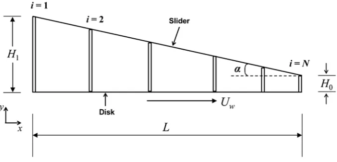
The channel geometry is represented by a series of micro-subdomain DSMC solvers that are distributed along the stream-wise flow direction as illustrated in Fig. 1 for the slider bearing geometry. These DSMC subdomains treat the physics fully in the cross-flow direction and inter-act indirectly with each other via constraints applied by a one-dimensional macroscopic mass conservation model constructed along the flow-direction. In the IMM, each subdomain state is predicted iteratively such that all sub-domains collectively satisfy the macroscopic mass conser-vation, subject to the correct boundary condition imposi-tion at the inflow and outflow of the channel geometry. The methodology for the DSMC subdomain simulations and the construction of the macroscopic mass conservation model is described next.

For carrying out the subdomain DSMC simulations, the local flow conditions (or equivalently the subdomain state) can be fully defined by: the gas density, 𝜌_i , the tangential wall velocity, U_w , and the stream-wise pressure gradient, 𝜙i . All micro-subdomains have exactly parallel walls cover-ing the full cross-section area of the channel at their local stream-wise location, x . A local parallel-flow assumption (valid for very low Reynolds number, gradually varying micro-channels where pressure differences along the stream-wise length of a thin micro subdomain can be neglected) allows subdomain DSMC simulations to be carried out with periodic boundary conditions (in the x-direction). The peri-odic simulations are enabled with the application of a cor-rection body force that emulates the effect of the missing pressure gradient. The DSMC subdomain simulations are thus carried out with the aid of a body force based on the pressure gradient correction, 𝜙i , which for an ideal gas can be expressed as:

where 𝜙i can be expressed as

(1) F_s,i= −𝜙i

𝜌_i

Fig. 1 _{Schematic of the IMM} configuration for the HDI gap (not to scale) with the slider at an angle 𝛼 degrees. Subdomain

The computed mass flow rate, mi from the subdomain DSMC simulations is fed as input to a macroscopic mass con-servation equation model for the entire geometry. The formula-tion of the macroscopic mass conservaformula-tion model is discussed next.

For the IMM iterative algorithm to be efficient, the varia-tion of the mass flow rate to changes in 𝜙_i and 𝜌_i needs to be expressed in the form of a general mass conservation equa-tion. For very low Reynolds number flows in gradually varying micro-channels, the velocity distribution, u(y), and hence the mass flow rate, m_i , can be related to the sum of the fundamen-tal individual flow components, i.e. Poiseuille, Couette and thermal creep flow components. Thermal creep effects can be ignored if there are no temperature variations along the chan-nel walls and isothermal conditions can then be assumed. The Couette flow rate component is independent of the Knudsen number, provided both walls have the same temperature and accommodation coefficient. On the other hand, the exact form of Poiseuille flow rate component is not known apriori and needs to be expressed as a function of the pressure gradient correction, 𝜙i . In the absence of any external acceleration, the Poiseuille flow component can be set to be proportional to the net momentum flux introduced by the pressure-gradient cor-rection. Thus, the total mass flow rate can be expressed as a function of the Couette flow and Poiseuille flow components as:

where Q_wall,i is the volumetric Couette flow rate component that is solely due to wall motion and k_i𝜙_i is the Poiseuille

flow rate due to the pressure gradient. The Poiseuille flow rate component is only approximate and the constants of proportionality, ki , can be estimated from Eq. (3) at the

beginning of the algorithm by performing either initial simu-lations with arbitrary values of 𝜌_i and 𝜙_i or from combina-tions of 𝜌i and 𝜙i which are previously known. In the present

work, excellent estimates of ki has been obtained from the initial iteration simulations with initialisation and ambient pressure boundary condition values relevant to the HDI gap problem. As discussed in Borg et al. (2015), the accuracy of these initial simulations and the obtained k_i values only determines the convergence characteristics of the method and does not affect the accuracy of the final IMM results. Equation (3) is then used to estimate the change in mass flow rate between successive iterations, n and n+1:

To make the mass flow rates in each subdomain tend toward a single mean value, mn_i+1 is replaced by M to obtain

(2) 𝜙i=

dp dx

(3) mi=𝜌iQwall,i−ki𝜙i

(4) mn+_i 1−mn_i =Q_wall,i(𝜌n+_i 1−𝜌n_i)+k_i(𝜙n_i −𝜙n+_i 1)

(5) M−Q_wall,i(𝜌_in+1−𝜌n_i)+k_i(𝜙n_i+1−𝜙n_i)−mn_i =0

Based on the equation of state for an ideal gas, Eq. (2) for 𝜙i can be re-written as

where R is the specific gas constant and T is the gas

tempera-ture. This allows Eq. (5) to be expressed as:

Equation (7) represents the one-dimensional macro-scopic mass conservation equation that needs to be solved iteratively. The solution of this macroscopic equation then provides the subdomain system states, 𝜌

i and 𝜙i , that is necessary for carrying out the DSMC micro-simulations to generate the mass flow rates, m_i , for the next IMM

iteration.

Thus, at each IMM iteration, the system of Eq. (7) for all subdomains need to be solved, subject to the imposition of pressure boundary conditions at the inflow and outflow of the channel to compute the unknowns, 𝜌_in+1 and M . In

the IMM configuration for the slider bearing, ambient pressure conditions (i.e. P₀ = 1 atm) exist and are imposed at the first and last subdomains. Accordingly, for a total of N subdomains, we have N equations and N + 1 unknowns (i.e. N unknown density values, 𝜌n+1

i , at the subdomain locations and the target mass flow rate, M , which is an

output of the IMM algorithm). The additional equation that is needed is obtained through the equation of state from the known (i.e. ambient) pressure boundary condition specified at the inflow or outflow.

At each iteration, the resulting system of equations (Eqs. 7, 8) for all subdomains can be solved using either a matrix inversion technique (e.g. LU decomposition) or an iterative method (e.g. Newton–Raphson). In this work, we have followed the Newton–Raphson iterative technique to obtain the solutions. Successively updated estimates of 𝜌i , mi , and 𝜙i are obtained at each IMM iteration until

macroscopic mass conservation is attained, at which the mass flow rate in each of the subdomains must be equal:

2.1.1 IMM algorithm

A schematic illustration of the IMM procedure is shown in Fig. 2. The various steps involved in the IMM algorithm are also summarised below:

(6)

𝜙_i=RTd𝜌

dx

| | | |

n+1

i

(7)

M−Qwall,i (

𝜌n_i+1−𝜌n_i)+kiRT (

d𝜌

dx | | | |

n+1

i

− d𝜌

dx | | | | n

i )

−mn_i =0

(8)

P_i=𝜌_iRT

(9)

1. Pre-simulation setup. Carry out initial simulations to ini-tialise all the subdomain states and get estimates of k_i for

each subdomain based on Eq. (3). The initial iteration is based on setting density states in all subdomains to a constant value subject to the correct pressure boundary condition imposition at the inflow and outflow.

2. For the first iteration, n=1 , carry out all

micro-subdo-main DSMC simulations with initial values of 𝜌n

i and 𝜙

n

i .

Extract the individual mass flow rate measurements, mn

i , from each subdomain simulation.

3. Use the current values of 𝜌n

i , 𝜙 n

i and m n

i to collectively solve the set of simultaneous equations (i.e. Equations 7, 8) using a suitable a matrix-inversion method or an iter-ative technique like the Newton–Raphson method. 4. Using updated values of pressure, 𝜌n+1_i and 𝜙n+1

i ,

obtained from step 3, carry out the sub domain simula-tions at n+1 to get a new estimate of the mass flow rate mn+1_i .

5. Repeat from (2) to get successively better updated val-ues of system states at each subdomain location and an improved estimate of the mass flux, until macroscopic mass conservation is attained (Eq. 9). The final IMM solution can now be obtained by extracting hydrody-namic variables like pressure, density, velocity, etc. from the DSMC subdomain simulations.

2.1.2 IMM numerical considerations

Two important aspects that need to be taken into considera-tion for the IMM are the choices for the spatial distribuconsidera-tion of subdomains and the discrete representation of the density gradient derivative term. These choices are dependent on the problem being considered. The discrete representation

of density in previous works (Patronis et al. 2013; Patronis and Lockerby 2014) was provided by the spectral colloca-tion scheme based on Fourier polynomials. Pseudo-spectral methods, although accurate, require nodes to be distributed carefully, i.e. nodes cannot be arbitrarily spaced. Subdo-mains typically need to be placed on Chebyshev nodes, as otherwise these result in undesirable oscillations at the limits of the intervals due to Runge’s phenomenon. In this work, the discrete representation of the density gradient derivative term in Eqs. (6) and (7) is enabled through a non-uniform grid finite difference method. The advantage of employ-ing the non-uniform grid FD method is the flexibility that it provides with respect to the distribution of subdomain locations. Particularly, for the slider bearing application con-sidered here, typical pressure profiles are characterised by a peak pressure and correspondingly large pressure gradient in a very small region towards the exit, while in the rest of the slider bearing only relatively small pressure gradients exist. Placing the majority of subdomains in the vicinity of relatively large density gradient regions (while keeping the number of subdomains elsewhere to a minimum) not only ensures optimal distribution of subdomains, but also greatly enhances the computational efficiency of the scheme as the total number of subdomains can be minimised.

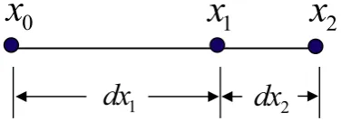
The non-uniform grid FD scheme (Fornberg 1988, 1998; Singh et al. 2009) used in this work is derived based on dif-ferentiating Lagrange’s interpolation polynomial scheme. Elegant and stable algorithms for obtaining the weights in FD formulas for arbitrary grids can be found in Fornberg’s work (1998), which derives simple recursions for calculating the weights of FD formulas for any order of derivative on one-dimensional grids with unequal spacing. As an example, for the first-order derivative involving the density gradient in Eq. (7), second-order accurate formulae for the central, forward and backward differencing terms based on three grid points, as shown in Fig. 3, can be expressed respectively as.

(10) f�(x₀) = −(2dx1+dx2)

dx1(dx1+dx2)

f₀+(dx1+dx2)

dx1dx2

f₁− dx1

dx2(dx1+dx2)

f₂

(11) f�(x₁) = −dx2

dx₁(dx₁+dx₂)f0−

(dx1−dx2)

dx₁dx₂ f1+

dx1

dx₂(dx₁+dx₂)f2 Fig. 2 A schematic illustration of the IMM

1

x

x

₂

0

x

1

dx

dx

2.2 Hybrid IMM‑DD methodology

The non-uniform-FD IMM described in Sect. 2.1 is capa-ble of simulating only internal micro-flows. In this work, we propose an IMM-DD hybrid that is capable of coupling internal flows modelled by IMM to domain decomposition type external regions outside the channel. For the slider bearing application considered in this study, the proposed hybrid method enables multi-scale modelling to couple rarefied internal flow regions within the HDI gap to con-tinuum flow outside the HDI region. The coupled model makes it possible to capture entrance and exit effects and study their impact on the HDI flow field. The hybrid method can also simulate localised heating effects due to instances like HAMR near the exit of the HDI gap, where no obvious degree of scale separation exists.

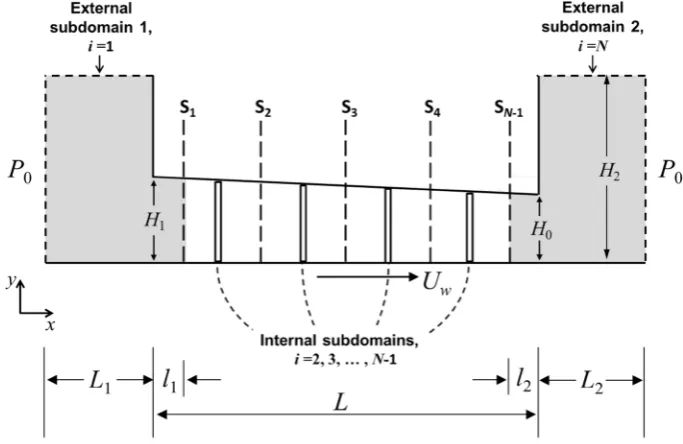
A schematic of the IMM-DD hybrid configuration is shown in Fig. 4. The hybrid HDI configuration consists of additional inflow and outflow regions of lengths L₁ and

L2 , respectively, in addition to the slider bearing

configura-tion of length, L . In this approach, there are several IMM micro-subdomains representing the internal flow within the HDI gap (referred to as internal subdomains). As in the IMM described in Sect. 2.1, the internal subdomains (i = 2, 3… N − 1) are periodic with parallel walls and can be non-uniformly distributed based on an irregularly-spaced finite difference method. Additionally, there are two extra sub-domains (shaded regions in Fig. 4), encompassing regions near the inflow and outflow. The two additional domains (12)

f�(x₂) = dx2

dx₁(dx₁+dx₂)f0−

(dx1+dx2)

dx₁dx₂ f1+

(dx1+2dx2)

dx₂(dx₁+dx₂)f2

(referred to as the external subdomains) are much larger and extend across a small internal flow region as shown in Fig. 4. The first external subdomain, i=1 , extends until

station S₁, while the second subdomain, i=N , extends from station S_N−1.

Our hybrid algorithm is an iterative scheme by which the internal subdomains are coupled to the external subdomains by essentially enforcing mass conservation to the pressure drop in the external subdomains and to the pressure gra-dient in the internal subdomains. Each of the subdomains (both internal and external) needs to have two stations over which the pressure difference/gradient can be defined. For the internal subdomains, the mass flow rate is related to the sum of the Couette and Poiseuille flow rates, as in Eq. (3). Equation (7) is then used to estimate the change in mass flow rate between successive iterations for the internal sub-domains based on the non-uniform grid FD method detailed in Sect. 2.1. The major difference with respect to the original IMM is in the placement of these subdomains relative to the stations at which the pressure is defined and solved. Sub-domains at which mass conservation equations are solved do not coincide with the pressure stations. Instead, they are staggered with respect to the pressure stations (S₁, S₂,…, S_N−1) as shown in Fig. 4, such that the pressure gradient across each internal subdomain can be defined. Accordingly, there are N − 1 stations (i.e. stations at which pressure is unknown and needs to be solved) for a total of N subdo-mains, as illustrated in Fig. 4. The correction body force representing the pressure gradient at each of the internal subdomain locations is now defined in terms of the pressure at these non-coincident pressure stations.

For the two external sections, a different set of mass balance equations are formed at stations, S₁ and S_N−1, by

relating the respective pressure drop over these two extra regions to the mass flow rates in each of them. Consequently, the mass balance equations at stations S₁ and SN−1 can be expressed respectively as Eqs. (13) and (14) given below

The constants of proportionality, ki , in Eqs. (13) and (14) can be estimated at the beginning of the algorithm either from pre-simulations or based on pressure solutions from the Reynolds gas lubrication equation for a faster convergence. The change in mass flow rate between successive iterations for the two external subdomains can now be expressed as

where M=mn+1

i to enable the mass flow rates in each

sub-domain to tend to a single macroscopic value. Equations (7), (15) and (16) represent the one-dimensional macroscopic mass conservation model for the hybrid IMM-DD that needs to be solved in conjunction with the DSMC subdomain simulations, at each iteration. The DSMC simulations pro-vide the mass flow rates, mn

i at the subdomain locations, the

methodology of which is described next.

The internal DSMC subdomain periodic simulations are carried out based on a correctional body force representing an effective pressure gradient, which is evaluated based on the non-uniform grid FD method detailed in Sect. 2.1. The modelling of external subdomains, however, needs care-ful consideration, as they are non-periodic with significant pressure gradients existing along the subdomains. Therefore, they cannot be simulated using an effective body force as in the case of the internal subdomains. We employ DSMC pressure boundary conditions to model the subsonic inflow and outflow of these special regions. Ambient pressure con-ditions, i.e. p=P₀ exist and are, therefore, imposed along the external boundaries of the external subdomains (denoted by dotted lines in Fig. 4). The IMM pressure solution at station S1 is imposed at the exit (outflow) of the first exter-nal subdomain, i=1 . Similarly, the IMM pressure solution obtained at station S_N is imposed at the inlet (inflow) of the second external subdomain, i=N . At these subsonic DSMC inflow and outflow boundaries, particles enter the domain from outside, the properties of which need to be determined appropriately. To fix the pressure boundary conditions, we have followed the subsonic characteristic boundary condi-tions (Wang and Li 2004), based on which, mainly the pres-sure is imposed, while other macroscopic flow properties at the boundaries are derived from the interior flow solution.

(13) m_i=𝜌_iQ_wall,i+k_i(P₁−P₀)

(14)

mi=𝜌iQwall,i+ki

(

P₀−P_N−1)

(15)

M−Q_wall,i(𝜌n+1 i −𝜌

n i

)

−k_i(Pn+_i 1−Pn_i)−mn i =0,

(16)

M−Q_wall,i

( 𝜌n+1

i −𝜌 n i

)

+k_i(Pn+1_i −Pn_i)−mn i =0,

The system of equations (i.e. Equation 7 for the internal subdomains and Eqs. (15) and (16) for the external sub-domains) is collectively solved using an iterative method (e.g. Newton–Raphson) to get new updated values of pres-sure at each station. For a total of N subdomains, including both internal and external regions, we have N equations and N unknowns (i.e. N − 1 unknown pressure values at the stations and the target mass flow rate, M , which is

an output of the IMM algorithm). Successively updated values of 𝜌_i , m_i , 𝜙_i , and Δp are obtained at each iteration

until mass conservation is attained.

2.3 Hybrid IMM‑DD algorithm

The steps involved in the hybrid IMM-DD are summarised below:

1. Initial setup. As in all IMM based methods, an initial iteration is carried out for initialisation of all the subdo-main states and to get estimates of k_i for each subdomain based on Eqs. (7), (15) and (16). The initial iteration is based on setting density states in all subdomains to an arbitrary value subject to the correct boundary condition imposition at the inflow and outflow.

2. For the current iteration, n , use the pressure values at each station to simulate all the subdomains. Carry out all internal periodic subdomain DSMC simulations with values of Pn

i and 𝜙 n

i estimated from the pressure stations based on the non-uniform grid FD method. The external subdomains are simulated with DSMC pressure bound-ary conditions using the pressure solution, Pn

i , at stations S₁ and S_N−1 and ambient pressure P₀ at the other external

boundaries. Obtain the individual mass flow rate meas-urements, mn

i , from each subdomain simulation. 3. Use the current values of Pn

i , 𝜙 n i and m

n

i to collectively solve the set of simultaneous equations (i.e. Equations 7, 15 and 16) using a suitable iterative technique like the Newton–Raphson method.

4. Obtain updated values of pressure, pn+1

i , at each of the stations and an overall mass flow rate prediction, M .

The updated pressure solution at stations S1 and SN−1, effectively couples the internal flow to the external flow by providing the necessary boundary condition to solve the external subdomains.

3 Results and discussion

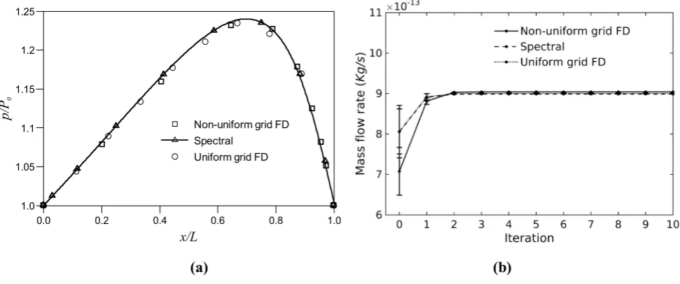
In this section, we apply the IMM and discuss the com-puted results for various HDI configurations. Before focus-sing on detailed validation of the IMM, we initially test and compare the accuracy of non-uniform-FD IMM solu-tions to corresponding IMM results from an evenly spaced finite-difference grid and the spectral collocation scheme (Patronis and Lockerby 2014). Comparisons have been done for a slider configuration of length L=5 μm, flying

height H₀=50 nm and disk wall velocity U_w=25 m/s . For this particular test case, we have employed a second-order slip solver for estimating the mass flow rate from the micro-subdomains. Ten subdomains have been employed for all cases. Comparisons of the pressure profiles com-puted by the three methods are shown in Fig. 5a. Excellent agreement is observed between the pressure profiles com-puted by all three methods. The convergence of the mean mass flow rate as a function of the IMM iteration number is shown in Fig. 5b. Error bars for the mean mass flow rate computed by the three methods are shown and the mean mass flow rate is computed as the average of the mass flow rate measurements from all the subdomains. The error bar is based on E=s∕√N where s is the standard

devia-tion and N is the total number of subdomains. Our results demonstrate that accurate results can be achieved using the non-uniform grid FD method, with the additional advan-tage and flexibility of clustering relatively more subdo-mains in regions of large pressure gradients (e.g. towards the exit region) for the same total number of subdomains.

Next, we focus on detailed validation of the IMM to compute flow in the vicinity of the HDI region. First, we

discuss the non-uniform grid FD IMM validation results for the slider bearing flow within the HDI region, i.e. with-out considering flow regions with-outside the slider. This will be followed by validation of the hybrid IMM-DD solutions that couple internal HDI regions to additional regions out-side the slider. In all cases, the IMM results have been val-idated against full-scale DSMC simulation results for the same flow configuration. All DSMC simulations (both full-scale DSMC as well as IMM subdomain atomistic solu-tions) have been carried out using the dsmcFoam + code (White et al. 2017). The dsmcFoam + code operates within the framework of the open source CFD code, OpenFOAM (2014), and has been validated for a wide range of bench-mark test cases (John et al. 2016; Palharini et al. 2015; Scanlon et al. 2010; White et al. 2017). To ensure accuracy of both our subdomain and full DSMC simulations, we have followed the established guidelines with respect to the cell size, time step, and particle numbers (Alexander et al. 1998; Hadjiconstantinou 2000; Hadjiconstantinou et al. 2003). The cell sizes in our study are defined to be much smaller than one-third of the mean free path, and an average of at least 50 particles has been considered in each cell. The time step for the DSMC simulations is taken to be five times smaller than Δx_min/ (V_mp+U_w) , where

Δx_min is the smallest cell dimension, Vmp is the most prob-able molecular velocity given by V_mp =√2R T_∞ , R is the

gas constant, T∞ is the reference temperature, and U_w is

the wall velocity.

3.1 IMM slider bearing results

We consider a slider bearing region of length, L=5

μm, pitch angle, 𝛼=0.01 rad and disk wall velocity,

(a) (b)

0.0 0.2 0.4 0.6 0.8 1.0

x/L

1.0 1.05 1.1 1.15 1.2 1.25

p/

P0

Non-uniform grid FD Spectral

Uniform grid FD

U_w=25 m/s . Four different cases of flying height, H₀ , are considered: 50 nm, 15 nm, 5 nm and 3 nm. The computed IMM solutions for pressure at different stream-wise loca-tions are compared with full-scale DSMC soluloca-tions in Fig. 6. The lower the flying height, the higher the peak pressure and higher loading capacity of the slider bearing. Correspond-ingly, the number of subdomains employed to capture the pressure gradient near the exit also varies depending on the flying height considered. The number of subdomains con-sidered varies from N = 6 for the H₀=50 nmcase to N = 10

for the case with H₀=3 nm . Excellent agreement can be observed between the full DSMC results and the IMM solu-tions for all cases considered.

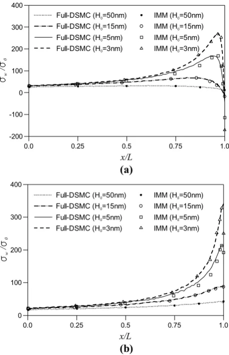
Next, we compare the computed wall shear stress values on both top (slider) and bottom (disk) walls. Shear stress gives important information about the forces acting on the walls. The wall shear stress has been computed based on the time-averaged tangential momentum exchange between the wall and the colliding molecules per unit time and area (Bird 1994). Comparison of the computed wall shear stress values between the full DSMC simulation and the IMM solutions for different cases of flying height is shown in Fig. 7. The wall shear stress, 𝜎_w in these plots is

non-dimensionalised with respect to the parameter, 𝜎₀ , where

𝜎₀=𝜇U_w∕L , 𝜇 , being the viscosity of the gas given by

𝜇=2.125×10−5Pa s at a reference temperature T =273 K .

Peak values of wall shear stress are observed towards the exit of the slider bearing where the peak pressure is also located. In general, for all cases of flying height consid-ered, the IMM solutions compare very well with the exact solutions, except at the exit of the channel (where the last subdomain is placed) where a discrepancy can be noted for the cases involving very small flying heights. This can be attributed to the fact that the peak pressure, which is several

times higher than the ambient pressure, is also very close to the exit for these cases. This makes ambient pressure bound-ary condition imposition at the outflow imprecise for the full DSMC simulation. The IMM on the other hand fixes the ambient conditions at the exit more exactly and hence the discrepancy between the two approaches.

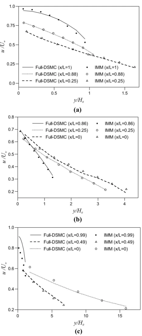
Finally, we compare the computed IMM velocity profiles across the channel height, at selected stream-wise locations along the channel. Validation is shown for three selected cases of H₀ in Fig. 8. It is to be noted that the subdomain

(stream-wise) locations in Fig. 8 varies for the different cases considered, since the total number of subdomains varies from N = 6 for the H₀=50 nm case to N = 10 for the case

with H₀=3nm . Good agreement can be observed for all

three cases at the different sections of the channel consid-ered. A discrepancy can be noted at the exit, particularly for the H₀=3 nm case. Again, this can be attributed to the

imprecise ambient outflow boundary condition imposi-tion for the full DSMC simulaimposi-tion, since the peak pressure

0.0 0.25 0.5 0.75 1.0

x/L

0 2 4 6 8 10

P/p0

Full-DSMC (H0=50nm) IMM (H0=50nm)

Full-DSMC (H0=15nm) IMM (H0=15nm)

Full-DSMC (H0=5nm) IMM (H0=5nm)

Full-DSMC (H0=3nm) IMM (H0=3nm)

Fig. 6 Comparison of the computed IMM pressure profile with full-scale DSMC solutions for the different cases of flying height consid-ered

(a)

(b)

0.0 0.25 0.5 0.75 1.0

x/L

-200 -100 0 100 200 300 400

w

/

0

Full-DSMC (H0=50nm) IMM (H0=50nm)

Full-DSMC (H0=15nm) IMM (H0=15nm)

Full-DSMC (H0=5nm) IMM (H0=5nm)

Full-DSMC (H0=3nm) IMM (H0=3nm)

0.0 0.25 0.5 0.75 1.0

x/L

0 100 200 300 400

w

/

0

Full-DSMC (H0=50nm) IMM (H0=50nm)

Full-DSMC (H0=15nm) IMM (H0=15nm)

Full-DSMC (H0=5nm) IMM (H0=5nm)

Full-DSMC (H0=3nm) IMM (H0=3nm)

location is very close to the channel exit for this case. This leads to minor discrepancies in the pressure drop at the exit of the channel when compared to the IMM which fixes the ambient conditions at the outflow more exactly.

3.2 Hybrid IMM‑DD results

Validation of the hybrid IMM-DD method has been demon-strated for four selected HDI configurations. The IMM-DD HDI configuration for the results discussed in this section follows the schematic shown in Fig. 4. Only selected results are shown for the sake of brevity. First, we test our hybrid method on the slider configuration of dimensions L = 5 μm,

H₀=50 nm, 𝛼=0.01 rad and U_w=25 m/s . For this test

case, we consider a total of ten subdomains. The dimen-sions of the external subdomains (i.e. L₁,H₁,L₂ and H₂ ) are

conservatively chosen such that their external boundaries are located sufficiently far away from the inflow and out-flow regions of the internal micro-out-flow domain. Accordingly, the external subdomain, i=1 , has dimensions L₁ = 1.5 μm,

H₂=1μm and also includes a small internal flow region

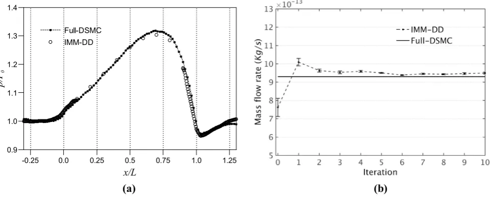
of length, l₁ = 0.5 μm, until station S₁ as shown in Fig. 4. Similarly, the external subdomain, i=N , has dimensions L₁ = 1.5 μm, H₂ = 1 μm and also includes a small internal flow region of length, l₂ = 0.5 μm, until station S_N−1. The internal subdomains are distributed non-uniformly between the external subdomains. The computed pressure profile from the IMM-DD solutions are validated against full-scale DSMC results and the comparison is shown in Fig. 9a. Good agreement between the solutions can be noted, with the pres-sure rise near the slider entrance region and prespres-sure drop near the exit of the slider well captured by the hybrid IMM solutions. The mean mass flow rate convergence as a func-tion of the IMM iterafunc-tion number for this case is shown in Fig. 9b, which converges to a constant value very quickly. Minor differences can be noted between the mass flow rates predicted by the full-scale DSMC and IMM-DD methods. However, the maximum error in the mass flow rate predicted by the IMM-DD method is consistently less than five percent from iteration number 2.

Additional validations for the hybrid IMM-DD method have also been carried out for exactly the same HDI region configuration as above, but with different flying heights, H₀=25 nm and H₀=15 nm . The results for the pressure

solution are shown in Fig. 10 and very good agreement can be observed between the IMM and the exact solutions, com-puted by full-scale DSMC, for both cases.

The next generation HDD’s require a flying height of the order of a few nanometers and modelling instances like par-ticle–surface interaction, asperity, localised heat generation due to HAMR, etc. will play a key role in determining accu-rate flow field conditions near the read/write head region. DSMC can be employed for a detailed investigation in any

(b) (a)

0 0.5 1 1.5

y/H0

0.0 0.25 0.5 0.75 1.0

U/

u

w

Full-DSMC (x/L=1) IMM (x/L=1) Full-DSMC (x/L=0.88) IMM (x/L=0.88) Full-DSMC (x/L=0.25) IMM (x/L=0.25)

0 1 2 3 4

y/H0

0.2 0.3 0.4 0.5 0.6 0.7 0.8

U/

u

w

Full-DSMC (x/L=0.86) IMM (x/L=0.86) Full-DSMC (x/L=0.25) IMM (x/L=0.25) Full-DSMC (x/L=0) IMM (x/L=0)

(c)

0 5 10 15

y/H0

0.2 0.4 0.6 0.8 1.0

U/

u

w

Full-DSMC (x/L=0.99) IMM (x/L=0.99)

Full-DSMC (x/L=0.49) IMM (x/L=0.49)

Full-DSMC (x/L=0) IMM (x/L=0)

Fig. 8 Computed IMM flow velocity profiles along the channel height at selected stream-wise locations, x∕L , for different cases

of flying height considered a H0=50 nm , b H0=15 nm , and c H0=3 nm . Comparison is made with the corresponding full-scale

such small selected region of interest to capture the true physics, while the rest of the slider bearing region can be modeled by the IMM. To demonstrate this coupling capa-bility, we now consider an IMM-DD hybrid simulation of a slider configuration involving localised heating that is resentative of HAMR. For this case, the localised heating pre-vents the use of the IMM throughout the gap. A total of six subdomains have been considered for this case. The external subdomain, i=1 , extends until station S₁ and has

dimen-sions, L₁ = 1 μm, l₁ = 0.5 μm, and H₂ = 1 μm, as shown in Fig. 4. Similarly, the external subdomain, i=N , extends until station SN−1 and has dimensions, L2 = 1 μm, l2 = 1 μm and H₂ = 1 μm. The slider bearing configuration considered here has dimensions L = 5 μm, H₀=25 nm, 𝛼=0.01 rad

and U_w=25 m/s . To mimic the HAMR heating effects, a

higher wall temperature of T_w=773 K is imposed on the bottom wall in a very small region of length 50 nm , near to

the exit of the slider. A uniform wall temperature distribu-tion has been assumed in the hot spot region for simplicity. Elsewhere, a constant temperature of T_w=273 K is

con-sidered on both upper and lower walls. The distribution of the imposed wall temperature boundary profile on the disk and the relative location of the hot spot are shown in Fig. 11.

The predicted pressure profile by the IMM-DD method is compared against full DSMC solutions in Fig. 12. The computed baseline pressure profile for the same

(a) (b)

-0.25 0.0 0.25 0.5 0.75 1.0 1.25

x/L

0.9 1.0 1.1 1.2 1.3 1.4

p/

P0

Full-DSMC IMM-DD

Fig. 9 Plots showing a validation of hybrid IMM-DD pressure profile with full-scale DSMC solution and b IMM-DD mass flow rate conver-gence. The error bars for the mean mass flow rate are also shown. The slider bearing region is located between, 0_<x∕L<1

-0.2 0 0.2 0.4 0.6 0.8 1 1.2 x/L

1.0 1.25 1.5 1.75 2.0 2.25 2.5 2.75 3.0

p/

P0

IMM-DD (H0=25nm)

Full-DSMC (H0=25nm)

IMM-DD (H0=15nm)

Full-DSMC (H0=15nm)

Fig. 10 Validation of the hybrid IMM-DD pressure profile with full DSMC solutions for HDI configurations with H0=25 nm and H0=15 nm

-0.2 0.0 0.2 0.4 0.6 0.8 1.0 1.2

x/L

200 300 400 500 600 700 800 900

Tw

(K

)

Wall temperature profile

T=273K

T=773K

Fig. 11 Wall temperature profile imposed on the disk (bottom wall) for simulating the localised heated spot associated with HAMR. The slider bearing region falls in the range 0_<x∕L<1 . The external sub-domain, i=1 , is located in the region ₋0.2_<x∕L<0.1 , whereas the external subdomain, i=N , is located in the region 0.8_<x∕L<1.2 . The heated region lies completely within the external subdomain,

configuration without any localised heating is also shown. It can be clearly observed that HAMR significantly alters the pressure profile with a higher peak pressure, leading to enhanced loading capacity of the slider bearing. Good agreement between the hybrid results and full-scale atom-istic solution is obtained. The pressure spike due to the hot spot is well captured by the hybrid method.

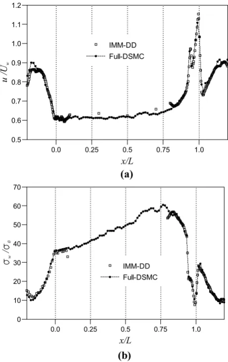
We have also computed the flow velocity and wall shear stress profiles along the disk surface represented by the bottom wall. Comparisons between the hybrid IMM-DD solutions and full-scale DSMC solutions for both these parameters are shown in Fig. 13. The wall shear stress, 𝜎_w , in Fig. 13b is nondimensionalised with respect

to the parameter, 𝜎₀ , where 𝜎₀=𝜇U_w∕L . The hybrid

solu-tions match closely with the exact solusolu-tions for both flow velocity and wall shear stress. Minor discrepancies can be noted at the entrance location (inflow) of the external subdomain. However, these are noted to be only local to the boundary. This can be attributed to the numerical arte-facts from the pressure boundary conditions at the cou-pled region. Therefore, some considerations need to be kept in mind while selecting the boundary of the external subdomain and imposing the pressure boundary condi-tion. It is recommended not to place the coupled boundary region too close to the pressure spike. Additionally, for the pressure boundary condition to be more exact and to minimise the related error, it is recommended to impose the boundary condition from volume reservoirs (Tysanner and Garcia 2005) rather than from surface reservoirs as is done typically.

3.3 IMM computational savings

The computational savings provided by the IMM mainly arises from two aspects. First, IMM requires significantly less cells and particles when compared to a full-scale DSMC solution. Second, the flow development time associated with a full-scale DSMC solution is substantially longer than the corresponding time needed for the IMM subdomains. An estimate on the computational savings, S , can be obtained using

where N_cell is the number of cells, P_cell , is the number of par-ticles per cell, T_d is the number of time steps it takes for flow

development (i.e. to reach steady state), T_av is the sampling (14)

S=

[

N_cellP_cell(T_d+T_av)]

Full

[

N_cellP_cell(T_d+T_av)]

IMM×Nit

0.0 0.25 0.5 0.75 1.0

x/L

1.0 1.2 1.4 1.6 1.8 2.0 2.2

p/

P0

Full-DSMC IMM-DD Baseline case

Fig. 12 _{Comparison of the computed hybrid IMM-DD pressure} pro-file with full-scale DSMC solutions for an HDI configuration involv-ing localised heatinvolv-ing on the bottom wall. Baseline case refers to the full DSMC solution for the same slider bearing configuration with-out any heating effects. The slider bearing region falls in the range

0<x_∕L<1

(a)

(b)

0.0 0.25 0.5 0.75 1.0

x/L

0.5 0.6 0.7 0.8 0.9 1.0 1.1 1.2

u

/Uw

IMM-DD Full-DSMC

0.0 0.25 0.5 0.75 1.0

x/L

0 10 20 30 40 50 60 70

w

/

0

IMM-DD Full-DSMC

period for time-averaging and N_it is the number of IMM

iterations required. For consistency, the same number of par-ticles per cell and sampling period are considered for both IMM and full-scale DSMC simulations to estimate S . For all

IMM slider bearing simulations reported in Sect. 3.1, IMM is about 15–20 times faster than a full-scale DSMC solu-tion. On the other hand, the IMM-DD simulations reported in Sect. 3.2 are only about 2–3 times faster than full-scale DSMC. For the hybrid simulations, the computational sav-ings predominantly comes from the reduced flow develop-ment time, as the subdomains reach steady state quickly compared to a full-scale solution. However, it is important to note that, while we have considered only representative slider lengths of 5 microns for validation purposes, realistic sliders have lengths of the order of a few millimetres. For such realistic slider bearing geometries, the estimated com-putational savings from the IMM will be at least two orders of magnitude.

4 Conclusions

A hybrid internal multi-scale method that is capable of mod-elling multi-scale flow in micro- and nano-devices has been presented. In particular, our model provides a framework to couple internal micro-flow regions modelled by the IMM approach to external flow regions modelled by a domain decomposition method. We have applied our hybrid IMM-DD approach to compute the flow field in the vicinity of the head-disk interface gap region in a hard disk drive enclosure. The internal flow regions within the HDI gap are modelled by the IMM based on a non-uniform grid finite-difference method to capture the strongly varying pressure gradient. The proposed hybrid method is then employed to couple internal micro-flows to the flow outside the HDI gap. In particular, cases involving localised heating effects in the HDI gap, where no obvious degree of scale separation exists, even within the HDI gap, can be modelled by our hybrid method. In all cases considered, the hybrid solutions are in good agreement with the full-scale DSMC solutions. Addi-tionally, the IMM is significantly faster than full DSMC solutions by about 15–20 times for the slider bearing simu-lations considered, whereas for the hybrid slider simusimu-lations the IMM is about 2–3 times faster. It is to be noted that for realistic HDI geometries, whose lengths are in the millimeter range, the estimated computational savings from the IMM will be at least two orders of magnitude.

To summarize, we have developed a novel hybrid IMM-DD multi-scale method that is capable of coupling the IMM to the domain decomposition method and applied it to the HDI gap problem. Although this work has focused on a particular application to demonstrate the capability of our method, the proposed hybrid approach can be easily applied

to simulate similar scale-separated multi-scale problems in other micro- and nano-devices. By suitably selecting the IMM subdomains and domain decomposition regions in a given problem, the hybrid method is capable of simulating very long micro-channels that can also have additional com-plexities like localised heating effects, asperities, additional inflow/outflow regions, etc. with substantial computational savings over a full-scale molecular solution.

Acknowledgements This work was supported through the United Kingdom Engineering and Physical Sciences Research Council under Grants EP/K038427/1, EP/K038664/1—“The First Open Source Soft-ware for Non-Continuum Flows in Engineering” and EP/N016602/1— “Nano-Engineered Flow Technologies: Simulation for Design across Scale and Phase”.

Open Access This article is distributed under the terms of the Crea-tive Commons Attribution 4.0 International License (http://creat iveco

mmons .org/licen ses/by/4.0/), which permits unrestricted use,

distribu-tion, and reproduction in any medium, provided you give appropriate credit to the original author(s) and the source, provide a link to the Creative Commons license, and indicate if changes were made.

References

Alexander FJ, Garcia AL, Alder BJ (1994) Direct simulation Monte Carlo for thin-film bearings. Phys Fluids 6:3854–3860

Alexander FJ, Garcia AL, Alder BJ (1998) Cell size dependence of transport coefficients in stochastic particle algorithms. Phys Fluids 10(6):1540–1542

Bahukudumbi P, Beskok A (2003) A phenomenological lubrication model for the entire Knudsen regime. J Micromech Microeng 13(6):873–884

Bhatnagar PL, Gross EP, Krook M (1954) A model for collision pro-cesses in gases. I. Small amplitude propro-cesses in charged and neu-tral one-component systems. Phys Rev 94:511–525

Bird GA (1994) Molecular gas dynamics and the direct simulation of gas flows. Clarendon Press, Oxford

Borg MK, Lockerby DA, Reese JM (2013a) A multiscale method for micro/nano flows of high aspect ratio. J Comput Phys 233:400–413

Borg MK, Lockerby DA, Reese JM (2013b) A hybrid molecular-continuum simulation method for incompressible flows in micro/ nanofluidic networks. Microfluidics Nanofluidics 15(4):541–557 Borg MK, Lockerby DA, Reese JM (2015) A hybrid molecular-contin-uum method for unsteady compressible multiscale flows. J Fluid Mech 768:388–414

Burgdorfer A (1959) The influence of the molecular mean free path on the performance of hydrodynamic gas lubricated bearings. ASME J Basic Eng 81:94–100

Cercignani C, Lampis M, Lorenzani S (2004) Variational approach to gas flows in microchannels. Phys Fluids 16:3426–3437

Cercignani C, Lampis M, Lorenzani S (2007) On the Reynolds equa-tion for linearized models of the Boltzmann operator. Transp Theory Stat Phys 36:257–280

Chen D, Bogy DB (2010) Comparisons of slip-corrected Reynolds lubrication equations for the air bearing film in the head-disk interface of hard disk drives. Tribol Lett 37(2):191–201 Fornberg B (1988) Generation of finite difference formulas on

Fornberg B (1998) Calculation of weights in finite difference formulas. SIAM Rev 40:685–691

Fukui S, Kaneko R (1988) Analysis of ultra-thin gas film lubrication based on linearized Boltzmann equation: first report-derivation of a generalized lubrication equation including thermal creep flow. ASME J Tribol 110(2):253–262

Fukui S, Kaneko R (1990) A database for interpolation of Poiseuille flow rates for high Knudsen number lubrication problems. ASME J Tribol 112(1):78–83

Gad-el-Hak M (1999) The fluid mechanics of microdevices—the Free-man scholar lecture. J Fluids Eng 121(1):5–33

Gad-El-Hak M (2006) MEMS: introduction and fundamentals. CRC Taylor and Francis

Gu XJ, Zhang H, Emerson DR (2016) A new extended Reynolds equa-tion for gas bearing lubricaequa-tion based on the method of moments. Microfluid Nanofluid 20(1):23

Hadjiconstantinou NG (2000) Analysis of discretization in the direct simulation Monte Carlo. Phys Fluids 12(10):2634–2638 Hadjiconstantinou NG (2005) Discussion of recent developments in

hybrid atomistic–continuum methods for multiscale hydrodynam-ics. Bull Pol Ac: Tech 53(4):335–342

Hadjiconstantinou NG, Garcia AL, Bazant MZ, He G (2003) Statisti-cal error in particle simulations of hydrodynamic phenomena. J Comput Phys 187(1):274–297

Hsia YT, Domoto GA (1983) An experimental investigation of molecu-lar rarefaction effects in gas lubricated bearings at ultra-low clear-ances. ASME J Lubr Tech 105(1):120–129

John B, Damodaran M (2009) Computation of head–disk interface gap micro flow fields using DSMC and continuum–atomistic hybrid methods. Int J Num Meth Fluids 61(11):1273–1298

John B, Gu XJ, Barber RW, Emerson DR (2016) High-speed rarefied flow past a rotating cylinder: the inverse Magnus effect. AIAA J 54(5):1670–1681

Lockerby DA, Duque-Daza CA, Borg MK, Reese JM (2013) Time-step coupling for hybrid simulations of multiscale flows. J Comput Phys 237:344–365

Myo KS, Zhou W, Huang X, Yu S, Hua W (2012) Slider posture effects on air bearing in a heat-assisted magnetic recording system. Adv Tribol 1–6

OpenFOAM: The open source CFD toolbox, user guide, version 2.3.1, 2014

Palharini RC, White C, Scanlon TJ, Brown RE, Borg MK, Reese JM (2015) Benchmark numerical simulations of rarefied non-reacting

gas flows using an open-source DSMC code. Comput Fluids 120:140–157

Patronis A, Lockerby DA (2014) Multiscale simulation of non-isother-mal microchannel gas flows. J Comput Phys 270:532–543 Patronis A, Lockerby DA, Borg MK, Reese JM (2013) Hybrid

con-tinuum-molecular modelling of multiscale internal gas flows. J Comput Phys 255:558–571

Ren W, Weinan E (2005) Heterogeneous multiscale method for the modeling of complex fluids and micro-fluidics. J Comput Phys 204(1):1–26

Scanlon TJ, Roohi E, White C, Darbandi M, Reese JM (2010) An open source, parallel DSMC code for rarefied gas flows in arbitrary geometries. Comput Fluids 39(10):2078–2089

Singh AK, Bhadauria BS (2009) Finite difference formulae for unequal subintervals using Lagrange’s interpolation formula. Int J Math Anal 3(17):815–827

Stephenson D, Lockerby DA, Borg MK, Nicholls WD, Reese JM (2015) Multiscale simulation of nanofluidic networks of arbitrary complexity. Microfluid Nanofluid 18:841–858

Tysanner MW, Garcia AL (2005) Non-equilibrium behavior of equilib-rium reservoirs in molecular simulations. Int J Num Meth Fluids 48:1337–1349

Wang M, Li Z (2004) Simulations for gas flows in microgeometries using the direct simulation Monte Carlo method. Int J Heat Fluid Flow 25(6):975–985

Weinan E, Engquist B, Huang Z (2003) Heterogeneous multiscale method: a general methodology for multiscale modelling. Phys Rev B 67:092101

Weinan E, Ren EW, Vanden-Eijnden W (2009) A general strategy for designing seamless multiscale methods. J Comput Phys 228(15):5437–5453

White C, Borg MK, Scanlon TJ, Longshaw S, John B, Emerson DR, Reese JM (2017) dsmcFoam+: an OpenFOAM based direct simu-lation Monte Carlo solver. Comput Phys Commun 224:22–43