warwick.ac.uk/lib-publications
Original citation:Yan, Ting, Jiang, Binyan, Fienberg, Stephen E. and Leng, Chenlei (2018) Statistical inference in a directed network model with covariates. Journal of the American Statistical Association. . doi:10.1080/01621459.2018.1448829
Permanent WRAP URL:
http://wrap.warwick.ac.uk/99216
Copyright and reuse:
The Warwick Research Archive Portal (WRAP) makes this work by researchers of the University of Warwick available open access under the following conditions. Copyright © and all moral rights to the version of the paper presented here belong to the individual author(s) and/or other copyright owners. To the extent reasonable and practicable the material made available in WRAP has been checked for eligibility before being made available.
Copies of full items can be used for personal research or study, educational, or not-for profit purposes without prior permission or charge. Provided that the authors, title and full bibliographic details are credited, a hyperlink and/or URL is given for the original metadata page and the content is not changed in any way.
Publisher’s statement:
“This is an Accepted Manuscript of an article published by Taylor & Francis in Journal of the American Statistical Association on 14/03/2018 available online:
https://doi.org/10.1080/01621459.2018.1448829
A note on versions:
The version presented here may differ from the published version or, version of record, if you wish to cite this item you are advised to consult the publisher’s version. Please see the ‘permanent WRAP URL’ above for details on accessing the published version and note that access may require a subscription.
Statistical Inference in a Directed Network Model with
Covariates
∗
Ting Yan
†Binyan Jiang
‡Stephen E. Fienberg
§Chenlei Leng
¶Abstract
Networks are often characterized by node heterogeneity for which nodes exhibit differ-ent degrees of interaction and link homophily for which nodes sharing common features tend to associate with each other. In this paper, we rigorously study a directed network model that captures the former via node-specific parametrization and the latter by in-corporating covariates. In particular, this model quantifies the extent of heterogeneity in terms of outgoingness and incomingness of each node by different parameters, thus allow-ing the number of heterogeneity parameters to be twice the number of nodes. We study the maximum likelihood estimation of the model and establish the uniform consistency and asymptotic normality of the resulting estimators. Numerical studies demonstrate our theoretical findings and two data analyses confirm the usefulness of our model.
Key words: Asymptotic normality; Consistency; Degree heterogeneity; Directed
net-work; Homophily; Increasing number of parameters; Maximum likelihood estimator.
1
Introduction
Most complex systems involve multiple entities that interact with each other. These
inter-actions are often conveniently represented as networks in which nodes act as entities and a
link between two nodes indicates an interaction of some form between the two corresponding
entities. The study of networks has attracted increasing attention in a wide variety of fields
including social networks (Burt et al., 2013; Lewisa et al., 2012), communication networks
(Adamic and Glance, 2005; Diesner and Carley, 2005), biological networks (Bader and Hogue,
∗Shortly after finishing the first draft of this paper, we were saddened to hear Steve Fienberg’s death. We
dedicate this work to his memory.
†Department of Statistics, Central China Normal University, Wuhan, 430079, China. Email:
‡Department of Applied Mathematics, Hong Kong Polytechnic University, Hong Kong.
Email:[email protected].
§Department of Statistics, Heinz College, Machine Learning Department, Cylab, Carnegie Mellon University,
Pittsburgh, PA 15213, USA.Email: [email protected].
¶Corresponding author. Department of Statistics, University of Warwick and Alan Turing Institute,
2003; Nepusz et al., 2012), disease transmission networks (Newman, 2002) and so on. Many
statistical models have been developed for analyzing networks in the hope to understand their
generative mechanism. However, it remains a unique challenge to understand the statistical
properties of many network models; for surveys, see Goldenberg et al. (2009), Fienberg (2012),
and a book long treatment of networks in Kolaczyk (2009).
Many networks are characterized by two distinctive features. The first is the so-called
degree heterogeneity for which nodes exhibit different degrees of interaction. In the language of
Barab´asi and Bonabau (2003), a typical network often includes a handful of high degree “hub”
nodes having many edges and many low degree individuals having few edges. The second
distinctive feature inherent in most natural and synthetic networks is the so-called homophily
phenomenon for which links tend to form between nodes sharing common features such as
age and sex; see, for example, McPherson et al. (2001). As the name suggests, homophily is
best explained by node or link specific covariates used to define similarity between nodes. As
a concrete example, we examine the directed friendship network between 71 lawyers studied
in Lazega (2001) that motivated this paper. The detail of the data can be found in Section
4. As is typical for interactions of this sort, various members’ attributes, including formal
status (partner or associate), practice (litigation or corporate) etc., are also collected. A
major question of interest is whether and how these covariates influence how ties are formed.
Towards this end, we plot the network in Figure 1 using red and blue colors to indicate different
statuses in (a) and black and green colors to represent lawyers with different practices in (b).
To appreciate the difference in the degrees of connectedness, we use node sizes to represent
in-degrees in (a) and out-degrees in (b). This figure highlights a few interesting features. First,
there is substantial degree heterogeneity. Different lawyers have different in-degrees and
out-degrees, while the in-degrees and the out-degrees of the same lawyers can also be substantially
different. This necessitates a model which can characterize the node-specific outgoingness and
incomingness. Second, ties seem to form more frequently if the vertices share a common status
or a common practice. As a result, a useful model should account for the covariates in order
to explain the observed homophily phenomenon.
This paper concerns the study of a generative model for directed networks seen in Figure
1 that addresses node heterogeneity and link homophily simultaneously. Although this model
is not entirely new, developing its inference tools is extremely challenging and we have only
started to see similar tools for models much simpler when homophily is not considered (Yan
Figure 1: Visualization of Lazega’s friendship network among 71 lawyers. The vertex sizes are proportional to either nodal in-degrees in (a) or out-degrees in (b). The positions of the vertices are the same in (a) and (b). For nodes with degrees less than 5, we set their sizes the same (as a node with degrees 4). In (a), the colors indicate different statuses (red for partner and blue for associate), while in (b), the colors represent different practices (black for litigation and green for corporate).
(a)
(b)
n ≥ 2 nodes labeled by 1, . . . , n. Let aij ∈ {0,1} be an indictor whether there is a directed
edge from node i pointing to j. That is, if there is a directed edge from i to j, then aij = 1;
otherwise, aij = 0. Denote A= (aij)n×n as the adjacency matrix of Gn. We assume that there
are no self-loops, i.e., aii = 0. Our model postulates that aij’s follow independent Bernoulli
distributions such that a directed link exists from node ito node j with probability
P(aij = 1) =
exp(Zij>γ+αi+βj)
1 + exp(Z>
ijγ+αi+βj)
.
In this model, the degree heterogeneity of each node is parametrized by two scalar parameters,
an incomingness parameter denoted by βi characterizing how attractive the node is and an
outgoingness parameter denoted byαi illustrating the extent to which the node is attracted to
others (Holland and Leinhardt, 1981). The covariate Zij is either a link dependent vector or a
function of node-specific covariates. If Xi denotes a vector of node-level attributes, then these
node-level attributes can be used to construct a p-dimensional vector Zij = g(Xi, Xj), where
g(·,·) is a function of its arguments. For instance, if we let g(Xi, Xj) equal to kXi −Xjk1,
our model, a larger Zij>γ implies a higher likelihood for node i and j to be connected. For the friendship network in Figure 1, for example, the covariate vector may include two covariates,
one indicating whether the two nodes share a common status and the other indicating whether
their practices are the same. Though similar models for capturing homophily and degree
heterogeneity have been considered by Dzemski (2014) for a general distribution function and
Graham (2017) in the undirected case, they focused on the homophily parameter and the
inference problem for degree heterogeneity was not studied. Because the formation of networks
is not only influenced by external factors (e.g., dyad covariates), but also affected by intrinsic
factors (e.g., the strengths of nodes to form network connection), it is statistically interesting
to conduct inference on the parameter associated with degree heterogeneity.
Model (1) assumes the independence of the network edges. As pointed out by Graham
(2017), the independent assumption may hold in some settings where the drivers of link
for-mation are predominately bilateral in nature, as may be true in some trade networks as well
as in models of (some types of) conflict between nation-states.
Since then(n−1) random variables ai,j,i6=j, are mutually independent given the
covari-ates, the probability of observing Gn is simply
n
Y
i,j=1;i6=j
exp (Zij>γ+αi+βj)aij
1 + exp(Zij>γ+αi+βj)
= exp X
i,j
aijZij>γ+α
>
d+β>b−C(α,β,γ), (1)
where
C(α,β,γ) =X
i6=j
log 1 + exp(Zij>γ+αi+βj)
is the normalizing constant. Here di =
P
j6=iaij denotes the out-degree of vertex i and
d = (d1, . . . , dn)> is the out-degree sequence of the graph Gn. Similarly, bj = Pi6=jaij
denotes the in-degree of vertex j and b = (b1, . . . , bn)> is the in-degree sequence. The
pair {b,d} or {(b1, d1), . . . ,(bn, dn)} is the so-called bi-degree sequence. As discussed before,
α= (α1, . . . , αn)>is a parameter vector tied to the out-degree sequence, andβ = (β1, . . . , βn)>
is a parameter vector tied to the in-degree sequence, and γ= (γ1, . . . , γp)> is a parameter
vec-tor tied to the information of node covariates. Since an out-edge from vertex i pointing toj is
the in-edge of j coming from i, it is immediate that the sum of out-degrees is equal to that of
in-degrees. If one transforms (α,β) to (α−c,β+c), the likelihood does not change. Because of this, for the identifiability of the model, we setβn = 0 as in Yan et al. (2016). Since we treat
are bounded. Therefore, the natural parameter space is
Θ ={(α>,β>1,...,n−1,γ>)> : (α>,β>1,...,n−1,γ>)>∈R2n+p−1},
under which the normalizing constant is finite.
Because of the form of the model and the independent assumption on the links, it appears
that maximum likelihood estimation developed for logistic regression is all that is needed for
inference. A major challenge of models of this kind is, however, that the number of parameters
grows with the network size. In particular, the number of outgoingness and incomingness
parameters needed by our model is already twice the size of the network, and the presence of
the covariates poses additional challenges. See the literature review below. To a certain extent,
our model can be seen as a special case of the exponential random graph model (ERGM) as
discussed by Robins et, al. (2007a,b), as the sufficient statistics are the covariates and the
bi-degree sequence. It is known, however, that fitting any nontrivial exponential random graph
models is extremely challenging, not to mention developing valid procedures for their statistical
inference (Goldenberg et al., 2009; Fienberg, 2012). Studying the asymptotic theory of the
proposed directed network model is the main contribution of this paper.
We empirically explore the asymptotic properties of the proposed estimators of the
hetero-geneity parameters α and β, as well as the homophily parameter γ. Our results demonstrate that the empirical study concur with our theoretical findings. Two real data examples are also
provided for illustration.
1.1
Literature review
Many network characteristics or configurations can be easily modeled as exponential family
distributions on graphs (Robins et, al., 2007a,b). For undirected networks, if we put the node
degrees as the sufficient statistics, then the model explains the observed degree heterogeneity
but not homophily. This model is referred to as the β-model by Chatterjee et al. (2011).
Exploring the properties of the β-model and its generalizations, however, is nonstandard due
to an increasing dimension of the parameter space and has attracted much recent interest
(Chatterjee et al., 2011; Perry and Wolfe, 2012; Olhede and Wolfe, 2012; Hillar and Wibisono,
2013; Yan and Xu, 2013; Rinaldo et al., 2013; Graham, 2017; Karwa and Slavkovi´c, 2016). In
estimator (MLE) and Yan and Xu (2013) derived the asymptotic normality of the MLE. In the
directed case, Yan et al. (2016) studied the MLE of a directed version of the β-model which
is a special case of the p1 model by Holland and Leinhardt (1981). Yan et al. (2016) did not
consider modelling homophily. By treating the node-specific parameters in the p1 model as
random effects, Van Duijn et al. (2004) proposed a random effects model incorporating nodal
covariates. The theoretical properties of the MLE of this model are difficult to establish and
thus have not been studied. Fellows and Handcock (2012) generalized exponential random
graph models by modeling nodal attributes as random variates. However, the theoretical
properties of their model are not explored. Hoff (2009) appears to be among the first to study
the model in (1). However, the theoretical properties of Hoff’s model are again unknown.
It is also worth noting that the consistency and asymptotic normality of the MLE have
been derived for two related models: the Rasch model (Rasch, 1960) for item response
exper-iments (Haberman, 1977) and the Bradley-Terry model (Bradley and Terry, 1952) for paired
comparisons by Simons and Yao (1999) in which a growing number of parameters are modelled.
The data for an item response experiment can be represented as a bipartite network and for
a paired comparisons data as a weighted directed network. None of these papers discussed
how to incorporate covariates. Finally, Model (1) can also be represented as a log-linear model
(Fienberg and Rinaldo, 2012). Although the necessary and sufficient conditions for the
exis-tence of the MLE for log-linear models with arbitrary dimension have been established [e.g.,
Haberman (1974); Fienberg and Rinaldo (2012)], there is lack of general results on the
asymp-totic properties of the MLE for high dimensional log-linear models as the analysis would be
challenging [Erosheva et al. (2007); Fienberg and Rinaldo (2007, 2012); Rinaldo et al. (2011)].
In the above mentioned network models, the dyads of network edges between two nodes
are assumed to be mutually independent. If network configurations such as k-stars and
tri-angles are included as sufficient statistics in the ERGMs, then edges are not independent and
such models incur the problem of model degeneracy in the sense of Handcock (2003), in which
almost all realized graphs essentially have no edges or are complete, completely skipping all
intermediate structures. Chatterjee and Diaconis (2013) have shown that most realizations
from many ERGMs look like the results of a simple Erdos-Renyi model and given a first
rig-orous proof of the degeneracy observed in the ERGM with the counts of edges and triangles
as the exclusively sufficient statistics. Yin (2015) further gave an explicit characterization
of the degenerate tendency as a function of the parameters. On the other hand, the MLE
(2013) demonstrated that the MLE is not consistent. In order to overcome the mode
degener-acy in ERGMs, Schweinberger and Handcock (2015) have proposed local dependent ERGMs
by assuming that the graph nodes can be partitioned intoK subsets (correspondingly,K
sub-graphs), in which dependence exists within subgraphs and edges are independence between
subgraphs. Based on this assumption, they established a central limit theorem for a network
statistic by referring to the Lindeberg–Feller central limit theorem whenK goes to infinity and
the number of nodes in subgraphs is fixed. The local dependency assumption essentially
con-tains a sequence of independent networks. On the other hand, some refined network statistics
such as “alternating k-stars”, “alternating k-triangles” and so on in Robins et, al. (2007b) are
proposed, but the theoretical properties of the model are still unknown. Moreover, Sadeghi
and Rinaldo (2014) formalized the ERGM for the joint degree distributions and derived the
condition under which the MLE exists.
The work close to our paper is Graham (2017) in which the β-model was generalized to
incorporate covariates to explain the homophily phenomenon and degree heterogeneity for
undirected networks. The asymptotic properties of a restricted version of the maximum
likeli-hood estimator were derived under the assumptions that all parameters are bounded and that
the estimators for all parameters are taken in one compact set. That is, his results are only
applicable to dense networks as pointed out in Graham (2017). In this paper, our focus is on
directed networks and our theory is established under more relaxed assumptions. In particular
the boundedness assumption on the parameters of degree heterogeneity in Graham (2017) is
not needed in our work. Hence our result covers more general networks. In addition, Graham
(2017) has focused on the consistency and the asymptotic normality of the parameter
estima-tor associated with covariates, while the asymptotic normality of the heterogeneity parameter
estimator was not studied. In this paper, we derive these two properties for the covariate
pa-rameter and the heterogeneity papa-rameters in model (1). It is worth remarking that establishing
the asymptotic normality for estimators of α and β is very challenging with the presence of the covariate Z. Graham (2016) further proposed a dynamic model to capture homophily
and transitivity when an undirected network over multiple periods is observed. The setup is
different from ours in that we only observe one network once. Moreover, Jochmans (2017)
developed a conditional-likelihood based approach to estimate the homophily parameter by
constructing a quadruple sufficient statistic to eliminate the degree heterogeneity parameter,
and further established the consistency and asymptotic normality of the resulting estimator.
con-sidered by Fern´andez-Val and Weidner (2016) and Cruz-Gonzalez et al. (2017) where time and
individual fixed effects are both considered. They focused mainly on the homophily parameter.
Dzemski (2017) applied the method in Fern´andez-Val and Weidner (2016) to a network model
similar to ours by including a scalar parameter to characterize the correlation of dyads. A
two-step approach was used for estimation and again the focus is on the homophily parameter.
There are major differences between these papers and ours including the methods of proofs,
the conditions required by the theorems and the attention to the degree parameters. We will
clarify these points after stating our main results in Section 3.
For the remainder of the paper, we proceed as follows. In Section 2, we give the details on
the model considered in this paper. In section 3, we establish asymptotic results. Numerical
studies are presented in Section 4. We provide further discussion and future work in Section
5. All proofs are relegated to the appendix.
2
Maximum Likelihood Estimation
We first introduce some notations. Let R = (−∞,∞) be the real domain. For a subset
C ⊂Rn, let C0 and C denote the interior and closure of C, respectively. For convenience, let
θ = (α1, . . . , αn, β1, . . . , βn−1)> and g = (d1, . . . , dn, b1, . . . , bn−1)>. Sometimes, we use θ and
(α,β) interchangeably. For a vector x= (x1, . . . , xn)> ∈Rn, denote by kxk∞ = max1≤i≤n|xi|
the `∞-norm of x. For an n×n matrix J = (Jij), let kJk∞ denote the matrix norm induced
by the `∞-norm on vectors in Rn, i.e.
kJk∞= max x6=0
kJxk∞ kxk∞
= max
1≤i≤n n
X
j=1
|Jij|.
The notation i < j < k is a shorthand for Pn
i=1
Pn
j=i+1
Pn
k=j+1. A “∗” superscript on a
parameter denotes its true value and may be omitted when doing so causes no confusion.
In what follows, it is convenient to define the notation:
pij(γ, αi, βj) =
exp(Zij>γ+αi+βj)
1 + exp(Zij>γ+αi+βj)
The log-likelihood of observing a directed network Gn under model (1) is
`(γ,α,β) = P
i6=j{aijlogpij(γ, αi, βj) + (1−aij) log(1−pij(γ, αi, βj))}
= P
i6=jaijZij>γ+
Pn
i=1αidi+
Pn
j=1βjbj −
P
i6=jlog(1 +e
Zij>γ+αi+βj).
(2)
The score equations for the vector parameters γ,α,β are easily seen as
P
i6=j
a
ijZ
ij=
P
i6=j Zije
Zij>γ+αi+βj
1+eZij>γ+αi+βj
,
d
i=
P
nk=1,k6=i
eZij>γ+αi+βk
1+eZij>γ+αi+βk
,
i
= 1
, . . . , n,
b
j=
P
nk=1,k6=j
eZ>ijγ+αk+βj
1+eZij>γ+αk+βj
, j
= 1
, . . . , n
−
1
.
(3)
The MLEs of the parameters are the solution of the above equations if they exist. LetK be
the convex hull of the set {(d>,b>1,...,n−1,
P
i,jaijZ
>
ij)> : aij ∈ {0,1},1 ≤ i 6= j ≤ n}. Since
the function C(α,β,γ) is steep and regularly strictly convex, the MLE of (α,β,γ) exists if and only if (d>,b>1,...,n−1,
P
i,jaijZ
>
ij)> lies in the interior of K[see, e.g., Theorem 5.5 in Brown
(1986) (p. 148)]. When the number of nodes n is small, we can simply use the R function
“glm” to solve (3). For relatively large n, this is no longer feasible as it is memory demanding
to store the design matrix needed forαandβ. In this case, we recommend the use of a two-step
iterative algorithm by alternating between solving the second and third equations in (3) via the
fixed point method in Yan et al. (2016) and solving the first equation in (3) via some existing
algorithm for generalized linear models.
In this paper, we assume that p, the dimension ofZ, is fixed and that the support ofZij is
Zp, where Z is a compact subset ofR. For example, if Zij’s are indictor variables such as sex,
then the assumption holds. For the parameters α and β, we make no such assumption and allow them to diverge slowly with n, the network size. To be precise, as long as kθ∗k∞, the
maximum entry of the true heterogeneity parameter, is bounded by a number proportional to
logn, our theory holds. See Theorem 1 for example. For technical reasons, it is more convenient
to work with the following restricted maximum likelihood estimators of α,β and γ defined as
(γb,αb,βb) = arg max γ∈Γ,α∈Rn,β∈Rn−1
`(γ,α,β), (4)
where Γ is a compact subset ofRpand
b
γ = (ˆγ1, . . . ,ˆγp)>,αb = ( ˆα1, . . . ,αˆn) >,
b
β = ( ˆβ1, . . . ,βˆn−1)>
the convex hull of the set constructed by all graphical bi-degree sequence (d>,b>1,...,n−1)> and
write (αb(γ),βb(γ)) = arg minα,β`(α,β,γ). For every fixed γ ∈ Γ, by Theorem 5.5 in Brown
(1986) (p. 148), the MLE (αb(γ),βb(γ)) exists if and only if (d>,b>1,...,n−1)> lies in the interior
of ˜K. Since Γ is a compact set, the restricted MLE exists if and only if (d>,b>1,...,n−1)> lies in
the interior of ˜K.
If γb lies in the interior of Γ, then it is also the global MLE of γ. Since we assume the dimension of Zij is fixed andγis one common parameter vector, it seems reasonable to assume
that kγkis bounded by a constant. If the restricted MLEs of αb andβbexist, they would satisfy
the second and third equations in (3). If γb ∈ Γ0, then it satisfies the first equation in (3).
Hereafter, we will work with the MLE defined in (4) and use “MLE” to denote “restricted
MLE” for shorthand.
3
Theoretical Properties
3.1
Characterization of the Fisher information matrix
The Fisher information matrix is a key quantity in the asymptotic analysis as it measures
the amount of information that a random variable carries about an unknown parameter of
a distribution that models the random variable. In order to characterize this matrix for the
vector parameter θ in our model (1), we introduce a general class of matrices that encompass the Fisher matrix. Given two positive numbers m and M with M ≥ m > 0, we say the
(2n−1)×(2n−1) matrixV = (vi,j) belongs to the class Ln(m, M) if the following holds:
m ≤vi,i−
P2n−1
j=n+1vi,j ≤M, i = 1, . . . , n−1; vn,n =
P2n−1
j=n+1vn,j,
vi,j = 0, i, j= 1, . . . , n, i6=j,
vi,j = 0, i, j=n+ 1, . . . ,2n−1, i6=j,
m ≤vi,j =vj,i≤M, i = 1, . . . , n, j =n+ 1, . . . ,2n−1, j 6=n+i,
vi,n+i =vn+i,i = 0, i= 1, . . . , n−1,
vi,i =
Pn
k=1vk,i=
Pn
k=1vi,k, i=n+ 1, . . . ,2n−1.
Clearly, if V ∈ Ln(m, M), then V is a (2n−1)×(2n−1) diagonally dominant, symmetric
nonnegative matrix and V has the following structure:
V =
V11 V12
V12> V22
,
where V11 ∈ Rn×n and V22 ∈ R(n−1)×(n−1) are diagonal matrices, V12 is a nonnegative matrix
whose non-diagonal elements are positive and diagonal elements equal to zero. One can easily
show that the Fisher information matrix for the vector parameter θ belongs to Ln(m, M) for
any γ ∈Γ. The exact form of this matrix can be found after Theorem 3 in Section 3.2. Thus, with some abuse of notation, we use V to denote the Fisher information matrix for the vector
parameter θ in the model (1). Define v2n,i = vi,2n := vi,i −
P2n−1
j=1;j6=ivi,j for i = 1, . . . ,2n −1 and v2n,2n =
P2n−1
i=1 v2n,i.
Then m ≤ v2n,i ≤ M for i = 1, . . . , n−1, v2n,i = 0 for i = n, n+ 1, . . . ,2n−1 and v2n,2n =
Pn
i=1vi,2n =
Pn
i=1v2n,i. Because of the special structure of any matrix V ∈ Ln(m, M), Yan et
al. (2016) proposed to approximate its inverse V−1 by the matrix S = (s
i,j), which is defined
as
si,j =
δi,j
vi,i +
1
v2n,2n, i, j = 1, . . . , n,
− 1
v2n,2n, i= 1, . . . , n, j =n+ 1, . . . ,2n−1,
− 1
v2n,2n, i=n+ 1, . . . ,2n−1, j = 1, . . . , n,
δi,j
vi,i +
1
v2n,2n, i, j =n+ 1, . . . ,2n−1,
(6)
where δi,j = 1 when i =j and δi,j = 0 when i6= j. They established an upper bound on the
approximation errors, stated in the lemma below.
Lemma 1. If V ∈ Ln(m, M) with M/m=o(n), then for large enough n,
kV−1−Sk ≤ c1M2
m3(n−1)2,
where c1 is a constant that does not depend on M, m and n, and kAk := maxi,j|ai,j| for a
general matrix A= (ai,j).
This lemma provides an accurate approximation of the inverse of the Fisher information
matrix in the limiting distribution of the MLE be explicit.
3.2
Asymptotic results
We first establish the existence and consistency of θb. The main idea of the proof is as follows.
For every fixed γ∈Γ, we define a system of functions
Fγ,i(θ) = di− n
X
k=1;k6=i
eZij>γ+αi+βk 1 +eZ>ijγ+αi+βk
, i= 1, . . . , n,
Fγ,n+j(θ) = bj − n
X
k=1;k6=j
eZ>ijγ+αk+βj 1 +eZij>γ+αk+βj
, j = 1, . . . , n, (7)
Fγ(θ) = (Fγ,1(θ), . . . , Fγ,2n−1(θ))>,
which are just the score equations for θ with γ fixed. Then we construct a Newton’s iterative sequence {θ(k+1)}∞
k=0 with initial value θ
(0), where θ(k+1) = θ(k)−[F0(θ(k))]−1F(θ(k)). If the
iterative converges, then the solution lies in the neighborhood ofθ0. This is done by establishing
a geometrically fast convergence rate of the algorithm with the initial value as the true value.
This technique is also used in Yan et al. (2016). We first present the consistency of the MLE bθ
for estimatingθ in the following theorem, whose proof is given in the supplementary material. Theorem 1. Assume that γ∗ ∈Γ0 and θ∗ ∈R2n−1 with kθ∗
k∞≤τlogn, where 0< τ <1/24
is a constant, and that A ∼ Pγ∗,θ∗, where Pγ∗,θ∗ denotes the probability distribution (1) on A
under the parameters γ∗ and θ∗. Then as n goes to infinity, with probability approaching one, the MLE θb exists and satisfies
kbθ−θ∗k∞ =Op
(logn)1/2e8kθ∗k∞ n1/2
=op(1).
Further, if θb exists, it is unique.
In order to prove the consistency of γb, we define a profile likelihood
`c(γ,θb(γ)) = X
i6=j
aijZij>γ+ n
X
i=1
αi(γ)di+ n
X
j=1
βj(γ)bj+
X
i6=j
log(1 +eZij>γ+αi(γ)+βj(γ)), (8)
where θb(γ) = arg maxθ`(γ,θ). It is easy to show that
E[`(γ,α,β)] =−
X
i6=j
DKL(pijkpij(γ, αi, βj))−
X
i6=j
where
DKL(pijkpij(γ, αi, βj)) =
X
i,j
pijlog
pij
pij(γ, αi, βj)
is the Kullback-Leibler divergence of pij(γ, αi, βj) from pij := pij(γ∗, α∗i, βj∗) and S(p) =
−plogp−(1−p) log(1−p) is the binary entropy function. Since the Kullback-Leibler
dis-tance is nonnegative, the function (9) attains its maximum value when γ =γ∗, α= α∗ and
β = β∗. On the other hand, since pij is a monotonic function on its arguments, (γ∗,α∗,β∗)
is a unique maximizer of the function E[`(γ,α,β)]. The main idea of proving the consistency of γb is to show that n−2|`(γ,α,β)−
E[`(γ,α,β)]| is small in contrast with the magnitude of n−2E[`(γ,α,β)], then the MLE approximately attains at the maximum of the function E[`(γ,α,β)]. The consistency of γb is stated formally below, whose proof is given in Section
6.1.
Theorem 2. Assume that γ∗ ∈ Γ0 and kθ∗k
∞ ≤ τlogn, where 0 < τ < 1/24 is a constant,
and that A∼Pγ∗,θ∗. Then as n goes to infinity, we have
b
γ −→p γ∗.
Next, we establish asymptotic normality of bθ, whose proof is given in the supplementary
mateiral. This is done by approximately representingθbas a function ofg= (d1, . . . , dn, b1, . . . , bn−1)>
with an explicit expression.
Theorem 3. Assume that γ∗ ∈Γ0 and A∼Pγ∗,θ∗. If kθ∗k∞≤τlogn, where τ ∈(0,1/44) is
a constant, then for any fixed k ≥ 1, as n → ∞, the vector consisting of the first k elements
of (bθ−θ ∗
) is asymptotically multivariate normal with mean 0 and covariance matrix given by
the upper left k×k block of S defined in (6).
Remark 1. By Theorem 3, for any fixedi, asn → ∞, the convergence rate of ˆθiis 1/v 1/2
i,i , whose
magnitude is between O(n−1/2ekθ∗k∞) and O(n−1/2) by inequality (6) in the supplementary
material.
Now we provide the exact form ofV, the Fisher information matrix of the vector parameter
θ. For i= 1, . . . , n,
vi,l = 0, l= 1, . . . , n, l6=i; vi,i= n
X
k=1;k6=i
vi,n+j =
eZij>γ+αi+βj (1 +eZij>γ+αi+βj)2
, j = 1, . . . , n−1, j 6=i; vi,n+i = 0
and for j = 1, . . . , n−1,
vn+j,i =
eZij>γ+αl+βj
(1 +eZ>ijγ+αl+βj)2, l= 1, . . . , n, l 6=j; vn+j,j = 0,
vn+j,n+j = n
X
k=1;k6=j
eZij>γ+αk+βj
(1 +eZij>γ+αk+βj)2, vn+j,i = 0, i= 1, . . . , n−1.
Let H be the Hessian matrix of the log-likelihood function `(γ,α,β) in (2) which can be represented as
H =
Hγγ Hγθ
Hγθ> −V
.
Following Amemiya (1985) (p. 126), the Hessian matrix of `c(γ∗,θˆ(γ∗)) is Hγγ+HγθV−1Hγθ>.
To state the form of the limit distribution of ˆγ, define
In(γ∗) =−
1
n(n−1)
∂2`c(γ∗,θˆ(γ∗)) ∂γ∂γ> =
1
n(n−1)(−Hγγ−HγθV
−1H>
γθ), (10)
whose approximate expression is given in (20), and I∗(γ) as the limit of In(γ∗) as n goes to
infinity.
Theorem 4. Assume that γ∗ ∈Γ0 and θ∗ ∈R2n−1 with kθ∗
k∞≤τlogn, where 0< τ <1/24
is a constant, and that A ∼ Pγ∗,θ∗. Then as n goes to infinity, the p-dimensional vector
N1/2(γˆ−γ∗) is asymptotically multivariate normal distribution with mean I∗−1(γ)B∗ and
co-variance matrix I−1
∗ (γ), where N =n(n−1) and B∗ is the bias term given in (24). Remark 2. The limiting distribution of γb is involved with a bias term
µ∗ = I−1
∗ (γ)B∗ p
n(n−1).
If all parameters γ and θ are bounded, then µ∗ = O(n−1/2). It follows that B∗ = O(1) and
(I∗)i,j = O(1) according to their expressions. Since the MLE γb is not centered at the true
parameter value, the confidence intervals and the p-values of hypothesis testing constructed
from γb cannot achieve the nominal level without bias-correction under the null: γ∗ = 0. This is referred to as the so-called incidental parameter problem in econometric literature [Neyman
due to the appearance of additional parameters. Here, we propose to use the analytical bias
correction formula: γbbc = γb−Iˆ−1B/ˆ p
n(n−1), where ˆI and ˆB are the estimates of I∗ and
B∗ by replacingγ and θ in their expressions with their MLEs γb and θb, respectively. Dzemski
(2014) also used this bias correction procedure, but his expression depends on projected values
of pair-wise covariates into the space spanned by degree parametersαi andβj under a weighted
least square problem and is not explicit. In the simulation in next section, we can see that
the correction formula offer dramatically improvements over uncorrected estimates and exhibit
the corrected coverage probabilities, in which those for uncorrected estimates are below the
nominal level evidently. See also Hahn and Newey (2004) and Fern´andez-Val and Weidner
(2016) for Jackknife bias correction for nonlinear panel models. But as discussed in Dzemski
(2014), this method is difficult to implement for network models. Moreover, Graham (2017)
described an iterated bias correction procedure, which may be numerically unstable and is not
guaranteed to converge as demonstrated in Juodis (2013).
Remark 3. There are three main differences between the results in Fern´andez-Val and Weidner
(2016) and those in our paper. First, for proving their asymptotic results, Fern´andez-Val and
Weidner (2016) used a projection method by projecting the pairwise covariates into the space
spanned by degree parameters αi and βj as a weighted least squares problem, while we use
an elementary method by approximating the inverse matrix of the Fisher information of the
degree parameters via an analytical expression. As a result, the asymptotic variances of the
estimators in Fern´andez-Val and Weidner (2016) depend on projected values not having closed
form expressions, while ours are explicit and easier to compute. We also note that the matrix
to approximate the inverse of the incidental parameter Hessian in Fern´andez-Val and Weidner
(2016) is diagonal while ours is not. Second, the asymptotic distribution of the MLE of the
incident parameters in αi and βj is not addressed in Fern´andez-Val and Weidner (2016). Note
that the properties of the incidental parameter estimators are more challenging than the fixed
dimensional parameterγdue to their increasing dimensions. Third, Fern´andez-Val and Weidner
(2016) assumed that all parameters are bounded while we consider an asymptotic setting to
allow the upper bound of the degree parameter to increase as the size of a network grows.
4
Numerical Studies
In this section, we evaluate the asymptotic results of the MLEs for model (1) through simulation
4.1
Simulation studies
Similar to Yan et al. (2016), the parameter values take a linear form. Specifically, we set
α∗i+1 = (n−1−i)L/(n−1) fori= 0, . . . , n−1 and letβi∗ =α∗i,i= 1, . . . , n−1 for simplicity. By
default,βn∗ = 0. We considered four different values forLasL∈ {0,log(logn),(logn)1/2,logn}.
By allowing the true value of α and β to grow with n, we intended to assess the asymptotic properties under different asymptotic regimes. Similar to Graham (2017) and Dzemski (2014),
each element of the p-dimensional node-specific covariate Xi is independently generated from
a Beta(2,2) distribution. The difference is that their papers considered p = 1 while in this
paper we set p= 2 by letting Zij = (|Xi1 −Xj1|,|Xi2−Xj2|)>. For the parameter γ∗, we let
it be (1,1.5)>. Thus, the homophily effect of the network is determined by a weighted sum of
the similarity measures of the two covariates between two nodes.
Note that by Theorems 3, ˆξi,j = [ ˆαi−αˆj−(α∗i−α
∗
j)]/(1/vˆi,i+ 1/vˆj,j)1/2, ˆζi,j = ( ˆαi+ ˆβj−α∗i−
βj∗)/(1/vˆi,i+ 1/vˆn+j,n+j)1/2, and ˆηi,j = [ ˆβi−βˆj−(βi∗−β
∗
j)]/(1/ˆvn+i,n+i+ 1/vˆn+j,n+j)1/2 are all
asymptotically distributed as standard normal random variables, where ˆvi,i is the estimate of
vi,i by replacing (γ∗,θ∗) with (γb,θb). Therefore, we assess the asymptotic normality of ˆξi,j, ˆζi,j
and ˆηi,j using the quantile-quantile (QQ) plot. Further, we also record the coverage probability
of the 95% confidence interval, the length of the confidence interval, and the frequency that
the MLE does not exist. The results for ˆξi,j, ˆζi,j and ˆηi,j are similar, thus only the results of ˆξi,j
are reported. The average and median values of bγ are also reported. Finally, each simulation is repeated 10,000 times.
We simulated networks with n = 100 or n = 200 and found that the QQ-plots for these
two network sizes were similar. Therefore, we only show the QQ-plots for n= 200 in Figure 2
to save space. In this figure, the horizontal and vertical axes are the theoretical and empirical
quantiles, respectively, and the straight lines correspond to the reference line y=x. In Figure
2, when L = 0 and log(logn), the empirical quantiles coincide well with the theoretical ones,
while there are notable deviations when L = (logn)1/2. When L = logn, the MLE did not
exist in all repetitions (see Table 1, thus the corresponding QQ plot could not be shown).
Table 1 reports the coverage probability of the 95% confidence interval for αi −αj, the
length of the confidence interval as well as the frequency that the MLE did not exist. As
we can see, the length of the confidence interval increases as L increases and decreases as n
increases, which qualitatively agrees with the theory. The coverage frequencies are all close to
−3 −1 0 1 2 3 −3 −2 −1 0 1 2 3 L = 0
(i,j)=(1,2)
−3 −1 0 1 2 3
−3 −2 −1 0 1 2 3
(i,j)=(n/2, n/2+1)
−3 −1 0 1 2 3
−3 −2 −1 0 1 2 3
(i,j)=(n−1, n)
−3 −1 0 1 2 3
−3 −2 −1 0 1 2 3 L = log(log(n))
−3 −1 0 1 2 3
−3 −2 −1 0 1 2 3
−3 −1 0 1 2 3
−3 −2 −1 0 1 2 3
−3 −1 0 1 2 3
−3 −2 −1 0 1 2 3 L = (log(n)) 1 /2
−3 −1 0 1 2 3
−3 −2 −1 0 1 2 3
−3 −1 0 1 2 3
[image:18.595.85.502.61.490.2]−3 −2 −1 0 1 2 3
Figure 2: The QQ plots of ˆv1ii/2(ˆθi−θi).
not exist and the coverage frequencies for pair (1,2) are higher than the nominal level; when
[image:18.595.77.520.623.743.2]L is logn, the MLE did not exist for all repetitions.
Table 1: The reported values are the coverage frequency (×100%) for αi−αj for a pair (i, j)
/ the length of the confidence interval / the frequency (×100%) that the MLE did not exist.
n (i, j) L= 0 L= log(logn) L= (logn)1/2 L= logn
100 (1,2) 94.82/1.20/0 97.02/2.62/0 99.80/3.80/90.04 N A/N A/100 (50,51) 94.76/1.20/0 95.79/1.86/0 96.98/2.37/90.04 N A/N A/100 (99,100) 94.84/1.20/0 95.21/1.44/0 96.38/1.57/90.04 N A/N A/100
200 (1,2) 95.18/0.84/0 96.31/1.96/0 98.64/3.05/45.08 N A/N A/100 (100,101) 94.33/0.84/0 94.88/1.36/0 94.99/1.72/45.08 N A/N A/100 (199,200) 95.08/0.84/0 94.78/1.02/0 94.95/1.12/45.08 N A/N A/100
b
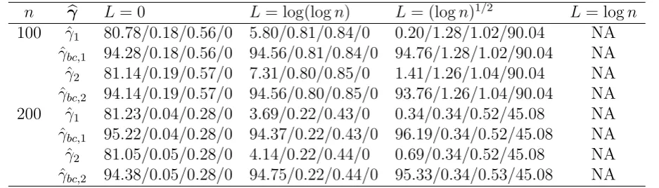
γbc(=γb−Iˆ−1B/ˆ p
n(n−1)) at the nominal level 95%, the average absolute bias as well as the
standard error. As we can see, the coverage frequencies for the uncorrected estimate is visibly
below the nominal level with at least 10 percentage points and the bias correction estimate
dramatically improve the coverage frequencies, whose coverage frequencies are close to the
nominal level when the MLE exists with a high frequency. On the other hand, whenn is fixed,
[image:19.595.65.534.246.380.2]the average absolute bias of γb increases as Lbecomes larger and so is the standard error. Table 2: The reported values are the coverage frequency (×100%) for γi for i / average bias
/ length of confidence interval /the frequency (×100%) that the MLE did not exist (γ∗ = (1,1.5)>).
n γb L= 0 L= log(logn) L= (logn)1/2 L= logn
100 ˆγ1 80.78/0.18/0.56/0 5.80/0.81/0.84/0 0.20/1.28/1.02/90.04 NA
ˆ
γbc,1 94.28/0.18/0.56/0 94.56/0.81/0.84/0 94.76/1.28/1.02/90.04 NA
ˆ
γ2 81.14/0.19/0.57/0 7.31/0.80/0.85/0 1.41/1.26/1.04/90.04 NA
ˆ
γbc,2 94.14/0.19/0.57/0 94.56/0.80/0.85/0 93.76/1.26/1.04/90.04 NA
200 ˆγ1 81.23/0.04/0.28/0 3.69/0.22/0.43/0 0.34/0.34/0.52/45.08 NA
ˆ
γbc,1 95.22/0.04/0.28/0 94.37/0.22/0.43/0 96.19/0.34/0.52/45.08 NA
ˆ
γ2 81.05/0.05/0.28/0 4.14/0.22/0.44/0 0.69/0.34/0.52/45.08 NA
ˆ
γbc,2 94.38/0.05/0.28/0 94.75/0.22/0.44/0 95.33/0.34/0.53/45.08 NA
4.2
Two data examples
The analysis of a Lazega’s dataset. We first analyze Lazega’s datasets of lawyers (Lazega, 2001),
downloaded from https://www.stats.ox.ac.uk/~snijders/siena/Lazega_lawyers_data.
htm. This data set comes from a network study of corporate law partnership that was carried
out in a Northeastern US corporate law firm between 1988 and 1991 in New England. We
focus on the friendship network among the 71 attorneys including partners and associates of
this firm. These attorneys were asked to name attorneys whom they socialized with outside
work. Naturally for a network of this sort, many covariates of each attorney were collected. In
particular, the collected covariates at the node level include formal status (partner or associate);
gender (man or woman), location in which they worked (Boston, Hartford, or Providence),
years with the firm, age, practice (litigation or corporate) and law school attended (harvard
and yale, or ucon, or others). We define the covariate for each dyad as a 7 dimensional
vector consisting of the differences between these 7 variables of the two individuals, where for
categorical variables, the difference is defined as the indicator whether they are equal, and for
continuous variable, the difference indicates their absolute distance. The directed graph of this
practice in (b). Although it may deem appropriate to treat the friendship relationship as
undirected, from Figure 1, we can see that the numbers of outgoing and incoming connections
for many individuals are dramatically different. As a result, we model the friendship network
[image:20.595.61.552.172.659.2]as a directed one.
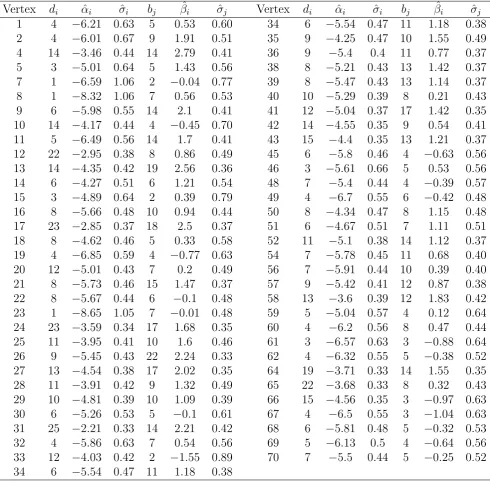
Table 3: The estimators of αi and βj and their standard errors in the Lazega’s data set.
Vertex di αˆi σˆi bj βˆi σˆj Vertex di αˆi σˆi bj βˆi σˆj
1 4 −6.21 0.63 5 0.53 0.60 34 6 −5.54 0.47 11 1.18 0.38 2 4 −6.01 0.67 9 1.91 0.51 35 9 −4.25 0.47 10 1.55 0.49 4 14 −3.46 0.44 14 2.79 0.41 36 9 −5.4 0.4 11 0.77 0.37 5 3 −5.01 0.64 5 1.43 0.56 38 8 −5.21 0.43 13 1.42 0.37 7 1 −6.59 1.06 2 −0.04 0.77 39 8 −5.47 0.43 13 1.14 0.37 8 1 −8.32 1.06 7 0.56 0.53 40 10 −5.29 0.39 8 0.21 0.43 9 6 −5.98 0.55 14 2.1 0.41 41 12 −5.04 0.37 17 1.42 0.35 10 14 −4.17 0.44 4 −0.45 0.70 42 14 −4.55 0.35 9 0.54 0.41 11 5 −6.49 0.56 14 1.7 0.41 43 15 −4.4 0.35 13 1.21 0.37 12 22 −2.95 0.38 8 0.86 0.49 45 6 −5.8 0.46 4 −0.63 0.56 13 14 −4.35 0.42 19 2.56 0.36 46 3 −5.61 0.66 5 0.53 0.56 14 6 −4.27 0.51 6 1.21 0.54 48 7 −5.4 0.44 4 −0.39 0.57 15 3 −4.89 0.64 2 0.39 0.79 49 4 −6.7 0.55 6 −0.42 0.48 16 8 −5.66 0.48 10 0.94 0.44 50 8 −4.34 0.47 8 1.15 0.48 17 23 −2.85 0.37 18 2.5 0.37 51 6 −4.67 0.51 7 1.11 0.51 18 8 −4.62 0.46 5 0.33 0.58 52 11 −5.1 0.38 14 1.12 0.37 19 4 −6.85 0.59 4 −0.77 0.63 54 7 −5.78 0.45 11 0.68 0.40 20 12 −5.01 0.43 7 0.2 0.49 56 7 −5.91 0.44 10 0.39 0.40 21 8 −5.73 0.46 15 1.47 0.37 57 9 −5.42 0.41 12 0.87 0.38 22 8 −5.67 0.44 6 −0.1 0.48 58 13 −3.6 0.39 12 1.83 0.42 23 1 −8.65 1.05 7 −0.01 0.48 59 5 −5.04 0.57 4 0.12 0.64 24 23 −3.59 0.34 17 1.68 0.35 60 4 −6.2 0.56 8 0.47 0.44 25 11 −3.95 0.41 10 1.6 0.46 61 3 −6.57 0.63 3 −0.88 0.64 26 9 −5.45 0.43 22 2.24 0.33 62 4 −6.32 0.55 5 −0.38 0.52 27 13 −4.54 0.38 17 2.02 0.35 64 19 −3.71 0.33 14 1.55 0.35 28 11 −3.91 0.42 9 1.32 0.49 65 22 −3.68 0.33 8 0.32 0.43 29 10 −4.81 0.39 10 1.09 0.39 66 15 −4.56 0.35 3 −0.97 0.63 30 6 −5.26 0.53 5 −0.1 0.61 67 4 −6.5 0.55 3 −1.04 0.63 31 25 −2.21 0.33 14 2.21 0.42 68 6 −5.81 0.48 5 −0.32 0.53 32 4 −5.86 0.63 7 0.54 0.56 69 5 −6.13 0.5 4 −0.64 0.56 33 12 −4.03 0.42 2 −1.55 0.89 70 7 −5.5 0.44 5 −0.25 0.52 34 6 −5.54 0.47 11 1.18 0.38
In the data set, individuals are labelled from 1 to 71. After removing those individuals
whose in-degrees or out-degrees are zeros, we perform the analysis on the 63 vertices left.
The minimum, 1/4 quantile, 3/4 quantile and maximum values of d are 1, 5, 8, 12 and 25,
respectively; those of b are 2, 5, 8, 13 and 22, respectively.
in which β71 = 0 is set as a reference. The estimates of heterogeneity parameters for
in-degrees and out-in-degrees vary widely: from the minimum −7.36 to maximum −1.68 for αbis
and from −1.32 to 2.56 for βbis. We then test three null hypotheses α1 = α4, α1 = β1 and
β1 =β4, using the proposed homogeneity test statistics ˆξi,j =|αˆi−αˆj|/(1/vˆi,i+ 1/ˆvj,j)1/2, ˆζi,j =
|αˆi−βˆj|/(1/vˆi,i+ 1/ˆvn+j,n+j)1/2, and ˆηi,j = |βˆi −βˆj|/(1/ˆvn+i,n+i + 1/vˆn+j,n+j)1/2 respectively.
The obtained p-values turn out to be 3.5× 10⁻⁴, 8.7×10⁻¹⁵ and 1.7×10⁻³, respectively,
confirming the need to use our model for parameterizing the in-degree and out-degree of each
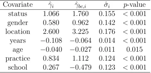
node differently to characterize the heterogeneity of bi-degrees. The estimated covariate effects,
their bias corrected estimators, their standard errors, and theirp-values under the null of having
no effects are reported in Table 4. The five categorial variables status, gender, location and
practice are all significant and positive, implying that a common value for any of these three
variables increases the likelihood of two lawyers to have connection. This is consistent with
Figure 1. On the other hand, the larger the difference between two lawyers’ age or their years
[image:21.595.176.422.406.524.2]with the firm, the less likely they are friends. This makes sense intuitively.
Table 4: The estimators ofγi, the corresponding bias corrected estimators, the standard errors,
and the p-values under the nullγi = 0 (i= 1, . . . ,7) for the Lazega’s friendship data.
Covariate ˆγi γˆbc,i σˆi p-value
status 1.066 1.760 0.155 <0.001 gender 0.580 0.962 0.142 <0.001 location 2.600 3.225 0.176 <0.001 years −0.108 −0.064 0.014 <0.001 age −0.040 −0.027 0.011 0.015 practice 0.834 1.112 0.124 <0.001
school 0.267 −0.479 0.123 <0.001
The analysis of Sina Weibo data. We now analyze the Sina Weibo data collected by Cai
et al. (2018). Sina Weibo is the largest Twitter-type social media in China. The original
data contains 4077 nodes in an official MBA program with directed edges representing who
follows who. For our analysis, we first remove those nodes with zero in-degrees or out-degrees
since in this case the MLEs of the corresponding degree parameters do not exist. The largest
strong connected subgraph of the remaining data set is then examined. This leaves a connected
network with 2242 nodes. The minimum, 1/4 quantile, 3/4 quantile and maximum values ofd
are 1, 2, 5, 19 and 715, respectively; those of b are 1, 4, 9, 22, 253, respectively. It exhibits a
strong degree heterogeneity.
Associated with each node are three variables: the number of characters in personal labels
posts (POST), and the time length since Weibo registration measured in months (TIME).
Be-fore our analysis, these node attributes are normalized by subtracting the average and dividing
their standard error. Then the covariates of edges are formed by using the absolute difference
distance.
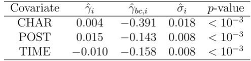
The two-step iterative algorithm in Section 2 is used to find the MLEs. The fitted values
of the homophily parameters using model (1) are summarized in Table 5. From this table, we
can see that all the node attributes are significant. In Figure 1 in the supplementary material,
the histograms of the fitted values of the degree parameters are provided. We can see that
the estimates of the heterogeneity parameters vary widely: from the minimum of −2.03 to the
maximum of 4.13 for ˆβj’s and from−8.87 to−1.28 for ˆαi’s. The histogram of ˆβj’s indicates that
[image:22.595.172.420.347.408.2]βj may follow a normal distribution while that of ˆαi’s clearly indicates a skewed distribution.
Table 5: The estimators ofγi, the corresponding bias corrected estimators, the standard errors,
and the p-values under the nullγi = 0 (i= 1,2,3) for the Sina Weibo data.
Covariate γˆi ˆγbc,i σˆi p-value
CHAR 0.004 −0.391 0.018 <10−3 POST 0.015 −0.143 0.008 <10−3
TIME −0.010 −0.158 0.008 <10−3
5
Discussion
In this paper, we have derived the consistency and asymptotic normality of the MLEs for
estimating the parameters in model (1) when the number of vertices goes to infinity. By allowing
kθ∗k∞ to diverge to infinity, our model can handle networks with the number of edges growing
with the number of node at a slow rate [Krivitsky et al. (2011)]. If the growth rate on the
degree parameters increases too fast, however, the MLE fails to exist with a positive frequency
as demonstrated in the simulation. Note that the conditions imposed on kθ∗k∞ in Theorems
1–4 may not be the best possible. In particular, the conditions guaranteeing the asymptotic
normality seem stronger than those guaranteeing the consistency. For example, the consistency
requires kθ∗k∞ ≤ 241 logn while the asymptotic normality requires kθ∗k∞≤ 441 logn. It would
be interesting to investigate whether these bounds can be improved.
There is an implicit yet strong assumption for our model that the reciprocity parameter
corresponding to the p1-model in Holland and Leinhardt (1981) is zero. However, if similarity
sharing similar node features. That would alleviate the lack of a reciprocity term to some
extent, although it would not induce reciprocity between dissimilar nodes. To measure the
reciprocity of dyads, it is natural to incorporate the model term ρP
i<jaijaji of thep1 model
into (1). In Yan and Leng (2015), encouraging empirical results were reported regarding the
distribution of the MLE in the p1 model without covariates. Nevertheless, although only one
new parameter is added, the problem of investigating the asymptotic theory of the MLEs
becomes more challenging. In particular, the Fisher information matrix for the parameter
vector (ρ, α1, . . . , αn, β1, . . . , βn−1) is not diagonally dominant and thus does not belong to the
class Ln(m, M). In order to apply the method of proofs here, a new approximate matrix with
high accuracy of the inverse of the Fisher information matrix is needed. On the other hand,
various extensions of the p1 model have been developed to allow the reciprocity parameters
to depend in a linear fashion on individuals i and j [Fienberg and Wasserman (1981)] and
block structures [Holland, Laskey and Leinhardt (1983); Wang and Wong (1987)]. Though
these models may be more realistic, their Fisher information matrices are no longer diagonally
dominant. As a result, investigating their asymptotic theory becomes much more involved and
we plan to do it in a future work.
Acknowledgements
We are very grateful to three referees, an associate editor, and the Editor Prof. Regina Liu
for their valuable comments that have greatly improved the manuscript. Our simulation code
is available on request. The authors thank Wei Cai at Northeast China Normal University for
sharing the Sina Weibo data. Yan’s research is partially supported by the National Natural
Science Foundation of China (No. 11771171). Jiang’s research is partially supported by the
Hong Kong RGC grant (PolyU 253023/16P). Leng’s research is partially supported by a Turing
Fellowship under the EPSRC grant EP/N510129/1.
References
Adamic, L. A. and Glance, N. (2005). The political blogosphere and the 2004 US Election.
Proceedings of the WWW-2005 Workshop on the Weblogging Ecosystem.
Amemiya, T. (1985). Advanced Econometrics. Cambridge, MA. Harvard University Press. Bader, G. D. and Hogue, C. W. V. (2003). An automated method for finding molecular
Barab´asi, A. L. and Bonabau, E. (2003). Scale-free networks. Scientific American, 50–59. Bradley, R. A. and Terry, M. E. (1952). The rank analysis of incomplete block designs I. The
method of paired comparisons. Biometrika, 39, 324–345.
Brown, L. D. (1986). Fundamentals of statistical exponential families with applications in statistical decision theory. Lecture Notes-Monograph Series. Hayward, California.
Burt, R. S., Kilduff, M., and Tasselli, S. (2013). Social Network Analysis: Foundations and
Frontiers on Advantage. Annual Review of Psychology,64, 527–547.
Cai, W., Guan, G., Pan, R., Zhu, X., and Wang, H. (2018). Network linear discriminant analysis. Computational Statistics & Data Analysis, 117, 32–44.
Chatterjee, S. and Diaconis, P. (2013). Estimating and understanding exponential random graph models. The Annals of Statistics, 41, 2428–2461.
Chatterjee, S., Diaconis, P., and Sly, A. (2011). Random graphs with a given degree sequence.
Annals of Applied Probability, 21, 1400–1435.
Cruz-Gonzalez, M., Fern´andez-Val, I., and Weidner, M. (2017). Probitfe and logitfe: Bias corrections for probit and logit models with two-way fixed effects. The Stata Journal, To
appear
Diesner, J. and Carley, K. M. (2005). Exploration of Communication Networks from the Enron Email Corpus. Proceedings of Workshop on Link Analysis, Counterterrorism and Security,
SIAM International Conference on Data Mining, 3–14.
Dzemski, A. (2014). An empirical model of dyadic link formation in a network with unobserved heterogeneity. Preprint. Available at http://pseweb.eu/ydepot/semin/texte1314/JMP\
%20ANDREAS\%20DZEMKI.pdf.
Dzemski, A. (2017). An empirical model of dyadic link formation in a network with unobserved heterogeneity. Working Papers in Economics, No 698.
Erosheva, E. A., Fienberg, S. E., and Joutard, C. (2007). Describing disability through individual-level mixture models for multivariate binary data. The Annals of Applied
Statis-tics, 1, 502–537.
Fellows, I. and Handcock, M. S. (2012). Exponential-family Random Network Models. Avail-able athttp://arxiv.org/abs/1208.0121.
Fienberg, S. E. (2012). A brief history of statistical models for network analysis and open
challenges.Journal of Computational and Graphical Statistics, 21, 825–839.
Fienberg, S. E. and Wasserman, S. S. (1981). Categorical data analysis of single sociometric relations. Sociological Methodology, 12, 156–192.
Fienberg, S. E. and Rinaldo, A. (2007). Three centuries of categorical data analysis: Log-linear models and maximum likelihood estimation. Journal of Statistical Planning and Inference,
137, 3430–3445.
Fienberg, S. E. and Rinaldo, A. (2012). Maximum likelihood estimation in log-linear models. The Annals of Statistics, 40, 996–1023.
Fern´andez-V´al, I. and Weidner, M. (2016). Individual and time effects in nonlinear panel
models with large N, T. Journal of Econometrics, 192, 291–312.
Goldenberg, A., Zheng, A. X., Feinberg, S. E., and Airoldi, E. M. (2009). A survey of statistical network models. Foundations and Trends in Machine Learning, 2, 129–233.
Econometrica, 85, 1033–1063.
Graham B. S. (2016). Homophily and transitivity in dynamic network formation. NBER
Work-ing Paper, No. 22186. Available at http://www.nber.org/papers/w22186.
Haberman, S. J. (1974). The Analysis of Frequency Data. Univ. Chicago Press, Chicago, IL. Haberman, S. J. (1977). Maximum likelihood estimates in exponential response models. The
Annals of Statistics, 5, 815–841.
Hahn, J. and Newey W. (2004). Jackknife and analytical bias reduction for nonlinear panel data models. Econometrica, 72, 1295–1319.
Handcock, M. S. (2003). Assessing degeneracy in statistical models of social networks, Working
Paper 39, Techenical report, Center for Statistics and the Social Sciences, University of Washington.
Hillar, C. and Wibisono, A. (2013). Maximum entropy distributions on graphs. Available at
http://arxiv.org/abs/1301.3321.
Hoeffding, W. (1963). Probability inequalities for sums of bounded random variables. Journal of the American Statistical Association, 58, 13–30.
Hoff, P. D. (2009). Multiplicative latent factor models for description and prediction of social
networks. Computational and Mathematical Organization Theory,15, 261–272.
Holland, P. W. and Leinhardt, S. (1981). An exponential family of probability distributions
for directed graphs (with discussion). Journal of the American Statistical Association, 76, 33–65.
Holland, P. W., Laskey, K. B., and Leinhardt, S. (1983). Stochastic blockmodels: First steps.
Social Networks.5, 109-137.
Jochmans, K. (2017). Semiparametric analysis of network formation. Journal of Business & Economic Statistics, To appear.
Juodis, A. (2013). A note on bias-corrected estimation in dynamic panel data models.
Eco-nomics Letters,118, 435–438.
Karwa, V. and Slavkovi´c, A. (2016). Inference using noisy degrees-Differentially private beta
model and synthetic graphs. The Annals of Statistics, 44, 87–112.
Kolaczyk, E. D. (2009).Statistical Analysis of Network Data: Methods and Models. New York, Springer.
Krivitsky, P. N., Handcock, M. S., and Morris, M. (2011). Adjusting for network size and
composition effects in exponential-family random graph models. Statistical Methodology, 8, 319–339.
Lazega, E. (2001). The Collegial Phenomenon: The Social Mechanisms of Cooperation Among
Peers in a Corporate Law Partnership.Oxford University Press, Oxford. Lang, S. (1993). Real and Functional Analysis. Springer.
Lewisa, K., Gonzaleza, M., and Kaufmanb, J. (2012). Social selection and peer influence in an
online social network.Proceedings of the National Academy of Sciences of the United States of America,109, 68–72.
Lo´eve, M. (1977). Probability theory I. 4th ed. Springer, New York.
McPherson, M., Lynn, S. L., and Cook, J. M. (2001). Birds of a feather: homophily in social
networks. Annual Review of Sociology,27, 415–444.
protein-protein interaction networks. Nature methods, 18, 471–472.
Newman, M. E. J. (2002). Spread of epidemic disease on networks. Physics Review E, 66,
016128.
Neyman, J. and Scott, E. (1948). Consistent estimates based on partially consistent observa-tions. Econometrica, 16, 1–32.
Olhede, S. C. and Wolfe, P. J. (2012). Degree-based network models. Available at http:
//arxiv.org/abs/1211.6537.
Perry, P. O. and Wolfe, P. J. (2012). Null models for network data. Available athttp://arxiv.
org/abs/1201.5871.
Rasch, G. (1960). Probabilistic Models For Some Intelligence And Attainment Tests. Copen-hagen: Paedagogiske Institut.
Rinaldo, A., Petrovi´c, S., and Fienberg, S. (2011). Maximum likelihood estimation in network
models. Technical report. Available at http://arxiv.org/abs/1105.6145.
Rinaldo, A., Petrovi´c, S., and Fienberg, S. E. (2013). Maximum likelihood estimation in the
β-model. The Annals of Statistics, 41, 1085–1110.
Robins, G., Pattison, P., Kalish, Y., and Lusher, D. (2007a). An introduction to exponential
random graph (p∗) models for social networks.Social Networks, 29, 173–191.
Robins, G., Snijders, T., Wang, P., Handcock, M., and Pattison, P. (2007b). Recent
develop-ments in exponential random graph (p*) models for social networks. Social Networks, 29, 192–215.
Sadeghi, K. and Rinaldo, A. (2014). Statistical models for degree distributions of networks,
NIPS 2014 Workshop “From Graphs to Rich Data”. Available at http://arxiv.org/abs/
1411.3825.
Schweinberger, M. and Handcock, M. S. (2015). Local dependence in random graph models:
characterization, properties and statistical inference.Journal of the Royal Statistical Society: Series B,77, 647–676.
Shalizi, C. R. and Rinaldo, A. (2013). Consistency under sampling of exponential random
graph models. The Annals of Statistics, 41, 508–535.
Simons, G. and Yao, Y. C. (1999). Asymptotics when the number of parameters tends to infinity in the Bradley-Terry model for paired comparisons. The Annals of Statistics, 27,
1041–1060.
Van Duijn, M. A. J., Snijders, T. A. B., and Zijlstra, B. J. H. (2004). p2: a random effects
model with covariates for directed graphs. Statistica Neerlandica, 58, 234–254.
Wang, Y. J. and Wong, G. Y. (1987). Stochastic blockmodels for directed graphs. Journal of the American Statistical Association, 82, 9–19.
Wu, N. (1997). The Maximum Entropy Method. New York, Springer.
Yan, T. and Leng, C. (2015). A simulation study of the p1 model. Statistics and Its Interface,
8, 255–266.
Yan, T., Leng, C., and Zhu, J. (2016). Asymptotics in directed exponential random graph
models with an increasing bi-degree sequence. The Annals of Statistics, 44, 31–57.
Yan, T. and Xu, J. (2013). A central limit theorem in the β-model for undirected random graphs with a diverging number of vertices. Biometrika, 100, 519–524.
Preprint. Available athttp://arxiv.org/abs/1512.06563.
6
Appendix: Proofs for theorems
In this section we give the proofs for Theorems 2 and 4 in Section 3, and the proofs for Theorems
1 and 3 are put in the online supplementary material.
6.1
Proof of Theorem 2
Recall thatθ= (α,β). In what follows, the calculations are based on the condition thatγ ∈Γ,
kθk∞≤nτ, whereτ ∈(0,1/2) is a positive constant. By calculations, we have
`(γ,θ) = `(γ,θ)−E[`(γ,θ)] +E[`(γ,θ)]
= X
i6=j
(aij −pij)(Zij>γ+αi+βj) +E[`(γ,θ)],
where E[`(γ,θ)] is given in (9) and pij =pij(γ∗, α∗i, βj∗). By the triangle inequality, we have
1
n(n−1)
n
X
i=1
X
j6=i
(aij−pij)Zij>γ
≤ 1 n n X i=1 1
n−1
X
j6=i
(aij −pij)Zij>γ
. (11)
Since we assume thatZij’s lie in a compact subset ofRp and the parameter space Θ of covariate
parameters is compact, we have for all i6=j,
max
γ∈Θ |Z
>
ijγ| ≤κ, (12)
whereκis a constant. By inequality (12),aijZij>γis a bounded random variable with the upper
bound κ. By Hoeffding’s (1963) inequality, we have
P
1
n−1
X
j6=i
(aij −pij)Zij>γ
≥
≤2 exp
−(n−1)
2
2κ2
.
By taking = 2κ[log(n−1)/(n−1)]1/2, we have
P
1
n−1
X
j6=i
(aij −pij)Zij>γ
≥2κ
s
log(n−1) (n−1)
!
≤ 4
Therefore, we have P 1
n(n−1)
n
X
i=1
X
j6=i
(aij −pij)Zij>γ
≥2κ
s
log(n−1) (n−1)
!
≤ P 1
n n X i=1 1
n−1
X
j6=i
(aij −pij)Zij>γ
≥2κ
s
log(n−1) (n−1)
! ≤ P n [ i=1 1
n−1
X
j6=i
(aij −pij)Zij>γ
≥2κ
s
log(n−1) (n−1)
!
≤ n
(n−1)2.
In the above, the first inequality is due to (11). Note that kαk ≤nτ and kβk ≤nτ. Similarly,
with probability at most n/(n−1)2, we have
1
n(n−1)
n
X
i=1
X
j6=i
(aij −pij)αi
≥
1
n(n−1)
n X i=1 X
j6=i
αi
n−1(aij −pij)
≥ 1
n(n−1)·n·n
τ
r
log(n−1)
n−1 =
(logn)1/2
n1/2−τ ,
and
1
n(n−1)
n
X
i=1
X
j6=i
(aij −pij)βj
≥
(logn)1/2
n1/2−τ .
Hence, with probability at least 1−3n/(n−1)2, we have
max
γ≤Γ,kθk∞≤nτ
1
n(n−1)
X
i
X
j6=i
(aij −pij)(Zij>γ+αi+βj)
<
(logn)1/2
n1/2−τ ,
or equivalently,
max
γ≤Γ,kθk∞≤nτ
1
n(n−1){`(γ,θ)−E[`(γ,θ)]}
<
(logn)1/2
n1/2−τ . (13)
Let Bn(ρ) = {γ : kγ−γ∗k∞ < ρ} be an open ball in Γ with γ∗ as its center and ρ as its
radius, and Bc
n(ρ) be its complement in Γ. Define
n(ρ) =
1
n(n−1)
max
kθk∞≤nτE
[`(γ∗,θ]− max
γ∈Bc
n(ρ),kθk∞≤nτE
[`(γ,θ)]
,
and
n(ρn) = arg min
ρ n(ρ)>
2(logn)1/2