Brain Decoding for Brain Mapping: Definition, Heuristic Quantification, and Improvement of Interpretability in Group MEG Decoding

(1)

DEPARTMENT OF INFORMATION ENGINEERING AND COMPUTER SCIENCE

ICT International Doctoral School

Brain Decoding for Brain Mapping

Definition, Heuristic Quantification, and

Improvement of Interpretability in Group MEG

Decoding

Seyed Mostafa Kia

International Doctorate School in Information

and Communication Technologies,

Universit`a degli Studi di Trento

Advisor:

Prof. Andrea Passerini

Universit`a degli Studi di Trento

(2)

(3)

Abstract

In the last century, a huge multi–disciplinary scientific endeavor is

de-voted to answer the historical questions in understanding the brain

func-tions. Among the statistical methods used for this purpose, brain decoding

provides a tool to predict the mental state of a human subject based on the

recorded brain signal. Brain decoding is widely applied in the contexts of

brain–computer interfacing, medical diagnosis, and multivariate hypothesis

testing on neuroimaging data. In the latest case, linear classifiers are

gen-erally employed to discriminate between experimental conditions. Then, the

derived weights are visualized in the form of brain maps to further study the

spatio–temporal patterns of the underlying neurophysiological activity. It is

well known that the brain maps derived from weights of linear classifiers

are hard to interpret because of high correlations between predictors, low

signal–to–noise ratio, across–subject variability, and the high

dimension-ality of the neuroimaging data. Therefore, improving the interpretability

of brain decoding approaches is of primary interest in many neuroimaging

studies. Despite extensive studies of this type, at present, there is no formal

definition for interpretability of multivariate brain maps. As a consequence,

there is no quantitative measure for evaluating the interpretability of

differ-ent brain decoding methods. In this thesis, as the primary contribution, we

propose a theoretical definition of interpretability in linear brain decoding;

we show that the interpretability of multivariate brain maps can be

decom-posed into their reproducibility and representativeness. As an application

of the proposed definition, we exemplify a heuristic for approximating the

interpretability in multivariate analysis of evoked magnetoencephalography

(MEG) responses. We propose to combine the approximated interpretability

and the generalization performance of the model into a new multi–objective

(4)

classifier based on the proposed criterion results in more informative

mul-tivariate brain maps. More importantly, the presented definition provides

the theoretical background for quantitative evaluation of interpretability,

and hence, facilitates the development of more effective brain decoding

al-gorithms in the future. As the secondary contribution, we present an

ap-plication of multi–task joint feature learning for group–level multivariate

pattern recovery in single–trial MEG decoding. The proposed method

al-lows for recovering sparse yet consistent patterns across different subjects,

and therefore enhances the interpretability of the decoding model. We

eval-uated the performance of the multi–task joint feature learning in terms of

generalization, reproducibility, and quality of pattern recovery against

tra-ditional single–subject and pooling approaches on both simulated and real

MEG datasets. Our experimental results demonstrate that the multi–task

joint feature learning framework is capable of recovering meaningful

pat-terns of varying spatio–temporally distributed brain activity across

indi-viduals while still maintaining excellent generalization performance. The

presented methodology facilitates the application of brain decoding for

char-acterizing the fine–level distinctive patterns of brain activity in group–level

inference on neuroimaging data.

Keywords

Brain Decoding; Brain Mapping; Neuroimaging; Machine Learning;

(5)

Acknowledgments

Firstly, I would like to express my sincere gratitude to my adviser Andrea

Passerini for his patience, constructive feedback, and support of my

re-search. Besides my advisor, I would like to thank the rest of my thesis

committee: Lauri Parkkonen, Alexandre Gramfort, and Lorenzo Bruzzone

for their insightful comments that improved this work significantly.

My special thanks also goes to Nathan Weisz for his ubiquitous

moti-vating attitude and valuable scientific supports. I owe a debt of gratitude

to Nicu Sebe and Paolo Giorgini, whose supports provided me the

oppor-tunity to continue my PhD study. I wish to thank James Haxby whose

lecture on “Neural Decoding” ignited the main motivation behind my

re-search activity.

I would like to thank my other collaborators and friends, Paolo Avesani,

Emanuele Olivetti, Sandro Vega Pons, Fabian Pedregosa, and Anna

Blu-menthal for stimulating discussions, criticisms, and kind feedback on the

content of this thesis.

Last but not the least, I would like to thank my family: my beloved wife

Nastaran, and my beloved parents Masood and Mina for their sympathetic

ear and spiritual supports throughout my life. I would like to dedicate this

(6)

(7)

List of Tables

2.1 Interpretation of the Bayes factor. . . 27

2.2 Some popular examples of the loss function. . . 32

2.3 Some popular choices for Ω. Here θi is used to refer to the

ith element of the parameter vector Θ. . . 35

3.1 Comparison between δΦ, ηΦ, and ζΦ for different λ values on the toy example shows the performance–interpretability

dilemma, in which the most accurate classifier is not the

most interpretable one. . . 76

3.2 The performance, reproducibility, representativeness, and

interpretability of ˆΦδ_i and ˆΦζ_i over 16 subjects. . . 82

3.3 The performance, reproducibility, representativeness, and

interpretability of ˆΦδ and ˆΦζ in the across–subject

decod-ing scenario. . . 89

(12)

decoding methods and the ground truth effect. The

num-bers show the average and the standard deviation of cosine

similarities between the ground–truth and brain maps in

10 simulation runs. The bold faced numbers show the best

method for each subject. The last row of the table shows the

mean similarity across subjects. MT-L21 maps are

signifi-cantly more representative of the ground–truth effect than

other benchmarked approaches. . . 119

A.1 Distribution of cosine similarity between two randomp-dimensional

vectors. . . 164

A.2 Cosine similarity between cERFs and APs across 16 subjects

and comparison between the generalization performance of

cERFs (δcERF), APs (δAP), and the weights of the decoding

model selected based on the proposed criterion (δζ). . . 167

(13)

List of Figures

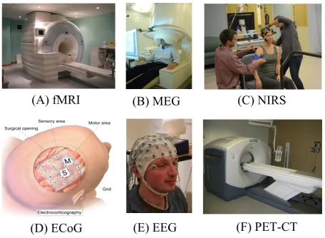
1.1 Neuroimaging techniques. (A) Siemens MAGNETOM Trio

device for structural and functional brain imaging. (B)

CTF–275 MEG scanner for recording magnetic fields

pro-duced by electrical currents in the brain. (C) User

prepa-ration for a NIRS recording. (D) A grid of ECoG sensors

implanted on sensory and motor areas. (E) Configuration

of EEG sensors on the head for scanning electrical brain

ac-tivity. (F) Discovery D600 PET–CT system for positron

emission tomography. . . 2

2.1 The structure of a typical neuron [206]. The electrical

sig-nals are received by the dendrites, processed at the soma,

and transmitted to the synaptic terminals via the axon. . . 15

2.2 (A) The organization of the white and gray matter in the

human brain. (B) The six layers of the gray matter. (C)

The division of human cerebral cortex into occipital,

pari-etal, temporal, and frontal lobes [204]. . . 16

2.3 The radial magnetic fields resulting from the tangential

elec-trical currents can be measured outside the scalp [205]. . . 18

2.4 Types of flux transformers in MEG sensors [68]: (A)

Mag-netometer, (B) Axial gradiometer, (C) Planar gradiometer. 19

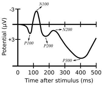
2.5 A schematic illustration of some well–known ERPs. . . 21

(14)

Fisher’s method for the significance testing. (B) Neyman–

Pearson’s method for the hypothesis testing. . . 25

2.7 The components of the error and the effect of regularization

on the bias and variance of a model [81]. . . 34

2.8 (A) In single–task learning the predictive functions are learned

independently across subject, while (B) multi–task learning

provides the possibility of sharing information across

differ-ent tasks in the learning process. . . 39

3.1 (A) The local co–occurrence rate of target words and

ma-chine learning related words. (B) The global co–occurrence

rate of target words and common intuitive definitions of

in-terpretability in brain decoding. . . 52

3.2 The high co–occurrence rate between the term

“Interpretabil-ity” with a variety of concepts such as “Stabil“Interpretabil-ity”,

“Repro-ducibility”, “Sparsity”, and “Plausibility” shows that there

is no consensus over its definition and quantification. . . . 53

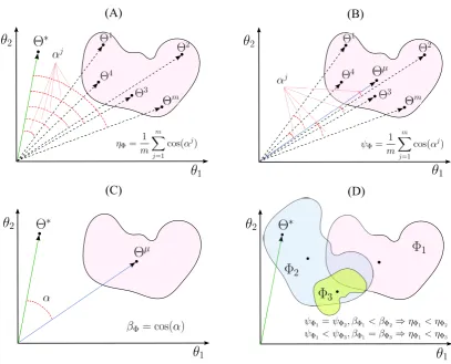
3.3 A schematic illustrations for (A) interpretability (ηΦ), (B) reproducibility (ψΦ), and (C) representativeness (βΦ) of a

linear decoding model in two dimensions. (D) The

indepen-dent effects of the reproducibility and the representativeness

of a model on its interpretability. . . 58

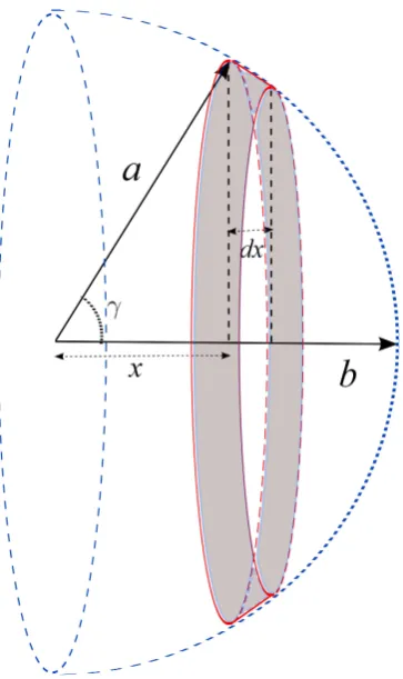
3.4 Two–dimensional geometrical illustration for computing the

PDF of cosine similarity. . . 60

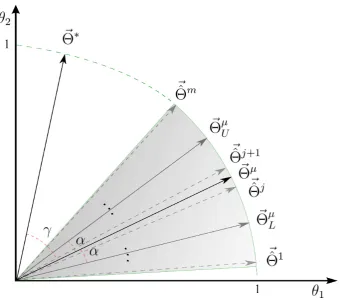
3.5 Relation between representativeness, reproducibility, and

in-terpretability in 2 dimensions. . . 65

(15)

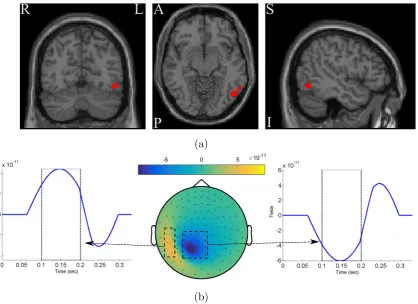
3.6 (A) The red circles show the dipole position, and the red

stick shows the dipole direction. (B) The spatio–temporal

pattern of the discriminative ground–truth effect. . . 73

3.7 Noisy samples of toy data. The dotted line shows the true

separator based on the generative model (Φ∗). The dashed line shows the most accurate classification solution. Because

of the contribution of noise, any interpretation of the

param-eters of the most accurate classifier yields a misleading

con-clusion with respect to the true underlying phenomenon [83]. 77

3.8 (A) The actual ηΦ, and (B) the heuristically approximated

interpretability ˜ηΦ of decoding models across different λ val-ues. There is a significant co–variation (Pearson’s

correla-tion p-value = 9×10−4) between ηΦ and ˜ηΦ. (C) The gen-eralization performance of decoding models. The box gives

the quartiles, while the whiskers give the 5 and 95 percentiles. 79

3.9 Topographic maps of weights of brain decoding models with

different λ values. . . 79

3.10 (A) Mean and standard–deviation of the performance (δΦ),

interpretability (ηΦ), and ζΦ of Lasso over 16 subjects. (B) Mean and standard–deviation of the reproducibility (ψΦ), representativeness (βΦ), and interpretability (ηΦ) of Lasso

over 16 subjects. The interpretability declines because of

the decrease in both reproducibility and representativeness

(see Proposition 1). (C) Mean and standard–deviation of

the bias, variance, and EPE of Lasso over 16 subjects. While

the change in bias is correlated with that of EPE (Pearson’s

correlation coefficient= 0.9993), there is anti–correlation

be-tween the trend of variance and EPE (Pearson’s correlation

coefficient=−0.8884). . . 81

(16)

and ˆΦζ_i. Adopting ζΦ instead of δΦ in model selection yields (on average) 0.04 less accurate classifiers over 16 subjects.

(B) Comparison between interpretabilities of ˆΦδ_i and ˆΦζ_i.

Adopting ζΦ instead of δΦ in model selection yields on

aver-age 0.31 more interpretable classifiers over 16 subjects. . . 83

3.12 Comparison between spatio–temporal multivariate maps of

(A)the most accurate, and(B) the most interpretable

clas-sifiers for Subject 1. Θ~ˆζ₁ provides a better spatio–temporal

representation of the N170 effect than Θ~ˆδ₁. . . 84

3.13 Comparison of the reproducibility of Lasso when δΦ and

ζΦ are used in the model selection procedure. (A) and (B) show the spatio–temporal patterns represented byΘ~ˆδ₁ across the 4 perturbed training sets. (C)and(D) show the spatio–

temporal patterns represented by Θ~ˆζ₁ across the 4 perturbed

training sets. Employing ζΦ instead of δΦ in the model

se-lection yields on average 0.15 more reproduciblilty of MBMs. 86

3.14 The mean and standard–deviation of the performance (δΦ),

interpretability (ηΦ), andζΦ of the elastic–net model over 16 subjects. In this dataset, increasing the amount of sparsity

increases the chance of performance–interpretability dilemma. 87

3.15 (A) Comparison between generalization performances of ˆΦδ_i

and ˆΦζ_i using elastic–net as the classifier. (B) Comparison

between the interpretability of ˆΦδ_i and ˆΦζ_i using elastic–net

as the classifier. The results obtained by the elastic–net

classifier are very similar to the Lasso model. . . 88

(17)

3.16 The spatio–temporal MBM of face processing in the across–

subject decoding scenario: (A) before the stimulus onset,

(B) 3 occipo–parietal dipoles 200 ms after the stimulus

on-set, (C) and (D) the forward ventral information flow from

300 to 400 ms after the stimulus onset, (E) the backward

information flow from temporal areas to occipital area 500

ms after the stimulus onset. . . 90

4.1 A schematic illustration for multi–task joint feature learning

via `2,1-norm. The resulting weight matrix has a similar sparse pattern across different tasks while each feature can

have different weights on different tasks. . . 108

4.2 (A) The dipole position in the RAS coordinate system (the

red circle). (B)The time–locked target effect is only present

in the trials of the positive class. (C) The background brain

activity is present in all simulated trials. (D) All trials are

contaminated with white Gaussian noise. (E) An example

of simulated trials in the positive and negative classes. . . 110

4.3 Comparison between the generalization performance and the

reproducibility of the 5 different methods on the simulated

and real MEG data. The results on the simulated data

are averaged over 10 simulation runs and 7 simulated

sub-jects. The results on the real MEG data are averaged over

16 subjects. MT-L21 provides the best decoding

perfor-mance, while preserving the highest reproducibility level

among other competing methods. . . 115

(18)

the weight vectors computed using 5 different decoding

ap-proaches (columns) on 7 simulated subjects (rows). The

weight vectors are normalized in the unit hyper–sphere. The

maps show the averaged weights in 100 ms interval from 100

to 200 ms after the stimulus onset. . . 116

4.5 Comparison between the temporal maps of the 5 different

decoding methods with the ground–truth effect, on data

from the first three simulated subjects. The time courses

are showing the temporal patterns of the recovered effect

computed by averaging the weights of the classifier over the

highlighted channels. The channels are selected based on

the spatial distribution of the dipole in the ground–truth

effect (see Figure 4.4). . . 118

4.6 A comparison between the reproducibility of spatio–temporal

maps in the SS-L1 and MT-L21 decoding approaches. The

topographic maps are plotted by averaging the weights of

the classifier between 100 and 200 ms in 3 simulation runs

of simulated subject 1. The recovered time courses are

plot-ted by averaging the weights over the highlighplot-ted channels.

MT-L21 is more stable in recovering the spatio–temporal

maps. . . 120

(19)

4.7 Comparison between the performance and reproducibility

of SS-L1, SS-L2, and MT-L21 across 16 subjects of real

MEG data. (A) The scatter plot of 16 decoding models

in the performance–reproducibility plane. The circles

repre-sent subjects and the colors denote different methods. (B)

The fitted normal distributions on the performance of 16

decoding models for 3 different approaches. (C) The fitted

normal distributions on the reproducibility of 16 decoding

models for 3 different approaches. . . 122

4.8 The recovered spatio–temporal representation of the N170

effect in 16 subjects from the real MEG dataset. The topoplots

show the classifier weights for magnetometer sensors

aver-aged in the 150 to 250 ms time period after stimulus onset.

The corresponding plots represent the temporal dynamic of

the dipole (red for the positive effect and blue for the

nega-tive effect) in the time dimension. . . 123

A.1 (A)The distribution of the sampled data without noise and

the true solution. (B) The distribution of sampled data

after noise contamination and the estimated solution of least

squares. . . 164

A.2 Histograms of cosine similarity between 10000 random

vec-tors with a random reference vector in p dimensional space. 166

A.3 (A)The clean positive sample. (B)A noisy positive sample

(C) A negative sample. . . 168

A.4 (A) The effect of sample size and on ∆β. Increase in

sample size and decrease in improves our approximation

of (B) representativeness and (C) interpretability. . . 169

(20)

sample size and decrease in σ improves our approximation

of (B) representativeness and (C) interpretability. . . 170

A.6 Recovered time course for simulated subject 4 using 5

dif-ferent methods. . . 170

A.10 Recovered topological maps using SS-L1 method from the

real MEG dataset across all 16 subjects. . . 172

A.11 Recovered topological maps using SS-L2 method from the

real MEG dataset across all 16 subjects. . . 173

A.12 Recovered topological maps using L1 (left) and

Pooling-L2 (Right) methods from the real MEG dataset. . . 173

(21)

Chapter 1

Introduction

Understanding the nature and function ofbrain is one of the main questions

that has evoked human curiosity all along the history. Ancient Greek

philosophers envisaged different functions for the brain from 500 B.C.E

to 200 C.E, ranging from it is being the cooling agent of body heat to

the seat of a rational soul and center of sensation and understanding [42].

Nowadays, cognitive science tries to incorporate research areas that are

concerned with neurophysiological and behavioral understanding of the

brain, e.g., neuroscience and psychology, with variety of other research

fields, such as computer science, physics, and statistics, to provide a better

insight into the structure and function of the brain. As the field matures,

techniques are being adopted from other areas of computational science in

order to accelerate research in cognitive science.

Neuroimaging techniques (see Figure 1.1), also called brain imaging

techniques, such as structural and functional Magnetic Resonance Imaging

(s/fMRI) [54], Electro/Magnetoencephalography (E/MEG) [20, 37],

Elec-trocorticography (ECoG) [103], Positron Emission Tomography (PET) [13],

and Near–Infrared Spectroscopy (NIRS) [25], have become essential tools

for either invasive or non–invasive imaging of the structure and function

of the brain. Structural brain imaging is more concerned about the

(22)

(A) fMRI

(B) MEG

(C) NIRS

(D) ECoG

(E) EEG

(F) PET-CT

Figure 1.1: Neuroimaging techniques. (A) Siemens MAGNETOM Trio device for struc-tural and functional brain imaging. (B) CTF–275 MEG scanner for recording magnetic fields produced by electrical currents in the brain. (C) User preparation for a NIRS recording. (D) A grid of ECoG sensors implanted on sensory and motor areas. (E) Con-figuration of EEG sensors on the head for scanning electrical brain activity. (F)Discovery D600 PET–CT system for positron emission tomography.

nosis of large–scale brain diseases resulting from the abnormality in brain

tissues [10, 179], e.g., tumors or brain injuries. On the other side, there

are a variety of applications for functional brain imaging, ranging from the

finer–level medical diagnosis to brain–computer interfaces and

understand-ing brain’s function.

In last three decades, the clinical application of functional brain

(23)

3 imaging techniques are used to investigate the neural correlates of various

mental disorders in order to identify biomarkers for them. These

biomark-ers then can be employed to investigate the effect of behavioral therapies

and drug treatments. For example, resting–state functional connectivity

derived from patients’ fMRI are used for early identification of Alzheimer’s

disease and presurgical planning [169]. MEG and EEG recordings are also

employed for finding the seizure onset zone in presurgical evaluation of

epilepsy patients [109].

Brain–computer interface [207] (BCI) is a system that provides a real–

time communication channel between the brain and an external machine.

The application of neuroimaging in BCI is more focused on measuring

elec-trical activity of brain invasively by means of intracranial implants such

as ECoG [120], or non–invasively by means of EEG devices. Then an

algorithm is used for online translation of the recorded brain activity to

machine instructions. This technology has applications in verbal

commu-nication [50], controlling devices [209], affect recognition [1–3, 110], multi–

media content retrival [59], and locomotion [200] especially for individuals

with severe motor disabilities by brainstem stroke or neuro–muscular

dis-eases such as amyotrophic lateral sclerosis.

In cognitive neuroscience [57], researchers use the recorded

neuroimag-ing data to understand the relationship between brain activity and specific

cognitive functions, i.e., to answer three key questions of where, when and

how 1 a brain region contributes to a particular cognitive process. To do this, depending on the question of interest, an experimental protocol is

designed to evoke or induce certain brain activity in human or non–human

participants, while simultaneously recording neural correlates by means of

functional neuroimaging devices. Then statistical analysis techniques are

1_{Here the answer to “how” question refers to finding the connection between a specific cognitive}

(24)

employed to justify the initial hypotheses about the three key questions.

Here is an example of a scientific question in cognitive neuroscience [140]:

“We here wanted to reveal whether neural excitability of the auditory

cortex putatively reflected in local alpha–band power is modulated already

prior to speech onset, and which brain regions may mediate such a top–

down preparatory response.”

in which auditory cortex, modulation of alpha–band power, and occurrence

of this modulation prior to speech onset stand for hypothesized answers to

where, how, and when questions, respectively.

In this thesis, we are interested in the application of functional

neu-roimaging in understanding brain function. More specifically, we are

inter-ested in improving the interpretability of multivariate hypothesis testing

approaches in order to infer more reliable, reproducible, and plausible

an-swers to the main questions in cognitive neuroscience. Of course, the

re-sulting methodology is also applicable to the medical diagnosis domain, but

our experimental setups and discussion are more focused on the

applica-tions in confirmatory and exploratory data analysis techniques in cognitive

neuroscience.

There are two schools of thought in statistical analysis for inference on

neuroimaging data [32]: 1) classical statistical testing, and 2) statistical

learning theory. Classical statistical testing is an in–sample

generaliza-tion technique based on null–hypothesis falsificageneraliza-tion, in which, generally,

a set of univariate tests, e.g., t–tests, are independently applied to each

variable of interest. On the other hand, statistical learning theory is a

multivariate approach that is more concerned with out–of–sample

gener-alization. While both techniques are successfully applied for inference on

neuroimaging data, they capture partially different aspects of the

underly-ing neurophysiological activity [32].

(25)

5 in classical inference on neuroimaging data [71, 160]. It is typically based

on the mean activity analysis, using e.g., ANOVA, on a pre–specified ROIs.

The pre–specified ROIs are generally decided using prior knowledge on the

studied cognitive process, and the mean activity within the ROIs are tested

in different experimental conditions. Despite the popularity and simplicity

of the ROI analysis method, the prerequisite for pre–selecting the ROIs

limits its application especially in exploratory analysis of neuroimaging

data where little is known about the brain areas involved in a cognitive

function. Addressing this limitation, classical inference evolved to the new

generation of exploratory whole–brain analysis such as mass–univariate

hypothesis testing [64].

Mass–univariate analysis performs a large number of univariate tests

on each variable, e.g., each voxel, independently. It can be employed for

hypothesis testing in whole–brain exploratory analysis without the need

for prior variable selection. However, it requires a procedure to handle

the multiple–comparison problem (MCP) [60]. There are various methods

for multiple–comparison correction based on the strong or weak control of

family–wise error rate (FWER) [203,213] or false discovery rate (FDR) [16]

control. Being essential for the validity of results, on the down side this

correction reduces the power of statistical analysis with the increase in the

number of univariate tests [64].

In statistical learning approaches, also known as brain decoding and

multivariate pattern analysis (MVPA) in the literature [86, 99], a model

is trained to learn the relation between the independent variables, i.e.,

neuroimaging data, and the dependent variables, i.e., experimental

condi-tions. The training is performed in the framework of statistical learning

theory [80]. The performance of the model is evaluated on a test set,

which is different from the initial training set. If the performance is

(26)

relation exists between the recorded neural signals and the cognitive task.

The statistical learning approach can possibly provide a multivariate

al-ternative for classical univariate hypothesis testing methods. The

multi-variate nature of this method yields higher sensitivity to the distributed

patterns of brain activities [149] and provides the possibility of

capitaliz-ing the complex interactions among the parameters of interest. Further,

by employing proper validation strategies, it resolves the multiple testing

problem of mass–univariate approaches [98]. In this thesis, we use brain

decoding to refer to the application of the statistical learning theory in the

neuroimaging context.

Due to the high dimensionality and limited number of samples typically

associated with neuroimaging data [41, 114], linear classifiers are generally

used to assess the relation between spatio–temporal brain measurements

and cognitive tasks [22, 118, 157]. This assessment is performed by

solv-ing an optimization problem that minimizes a loss function by learnsolv-ing

weights associated with each independent variable. These learned weights

can then be visualized in the form of a brain map, in which the

engage-ment of different brain areas in a cognitive task is illustrated. In fact,

brain mapping via brain decoding can be viewed as a pattern recovery

problem, where the goal is to recover spatio–temporal patterns of the

dis-criminative brain activity involved in the cognitive processing of external

stimuli. If successful, brain maps created by means of brain decoding can

provide a comprehensive explanation regarding the nature of neural

rep-resentations and brain states, and may be more informative for cognitive

science than a merely decoding accuracy measure [154]. Currently, brain

decoding is the gold standard in multivariate analysis of functional

mag-netic resonance images (fMRI) [41, 86, 135, 149] and

magnetoencephalogra-phy/electroencephalography(MEG/EEG) data [3, 34, 36, 93, 156, 167, 199].

(27)

7 interpretability of weights of classifiers, especially in group studies of

neu-roimaging data.

A classifier or a regression model that is trained in the statistical

learn-ing framework only answers the question of what is the most likely label

of a given unseen sample [12]. This fact is generally known as the

knowl-edge extraction gap [198] in the machine learning context. Thus far, much

effort has been devoted to filling this gap of linear and non–linear data

modeling methods in different areas such as computer vision [11], signal

processing [137], chemometrics [216], bioinformatics [72], and

neuroinfor-matics [83]. In the context of neuroimaging, this gap is generally known

as the interpretation problem [88, 142, 172]. Therefore, improving the

in-terpretability of linear brain decoding and the associated brain maps is a

topic of interest in many neuroimaging studies [178]. In spite of the

exten-sive efforts to improve the interpretability of brain decoding, there is still

no formal definition for the interpretability of brain decoding. Therefore,

the interpretability of different brain decoding methods is evaluated either

qualitatively or indirectly by means of an intermediate property.

Group–level analyses of neuroimaging data are extremely important,

as they allow for results to be generalized to new individuals. In

sta-tistical learning, an ideal group–level approach should be able to recover

both structural and functional similarities and dissimilarities across

differ-ent individuals. These similarities and dissimilarities generally occur at

both a coarse and fine level in space and time, and can provide valuable

spatio–temporal information about both the underlying macro and micro–

structures of the cognitive function in question. For example, visual stimuli

in general evoke a coarsely similar effect in early visual brain areas across

different subjects, but the response to different types or categories of visual

stimuli can differ from subject to subject at the finer level (see Ref. [87] for

(28)

level inference on neuroimaging data challenging, particularly since there is

also substantial across–subject variability in the brain structure (e.g., the

different size and shape of brains) [129, 164, 165, 180, 181]. This problem is

even more pronounced when one takes into account the difference in the

spatio–temporal structure of noise that commonly occurs due to different

external and internal sources, or manual preprocessing errors. These

vari-ations not only negatively affect the generalization performance of brain

decoding, but they also make post–hoc interpretation of the derived brain

maps more challenging, due to concerns about lack of reproducibility and

plausibility. For these reasons, it is crucial to explore more effective

de-coding methods that are capable of recovering structural and functional

similarities and dissimilarities in a group–level analysis of neuroimaging

data.

With the aim of filling these gaps, the contribution of this thesis is

two–fold:

1. A theoretical definition for the interpretability of linear brain

decod-ing models is presented. The definition is based on cosine proximity

between the estimated and true solutions of brain decoding in the

parameter space. Furthermore, it is shown that the interpretability

can be decomposed into the reproducibility and representativeness.

As a proof of concept, a practical heuristic based on event–related

fields is exemplified to quantify the interpretability of brain maps.

Furthermore, the combination of interpretability and performance of

brain decoding is proposed as a new Pareto optimal multi–objective

criterion for model selection.

2. An application of multi–task joint feature learning [9] for accurate

spatio–temporal pattern recovery at the group–level decoding of MEG

(29)

9 is considered as a task in the multi–task learning framework, where

only one decoding model is simultaneously trained over all subjects.

Further, `2,1 regularization [124] is employed to learn sparse patterns

consistently across different subjects, i.e., to jointly learn the features

across different subjects.

Regarding my first contribution, the presented definition for

interpretabil-ity of linear brain decoding models provides a concrete framework for a

pre-viously abstract concept and establishes theoretical background to explain

an ambiguous phenomenon in the brain decoding context. The

experi-mental results on MEG data show that accounting for the approximated

measure of interpretability has a positive effect on the human

interpreta-tion of brain decoding models. Furthermore, the proposed decomposiinterpreta-tion

of the interpretability of brain maps into their reproducibility and

repre-sentativeness explains the relationship between the influential cooperative

factors in the interpretability of brain decoding models and highlights the

possibility of indirect and partial evaluation of interpretability by

mea-suring these effective factors. The experimental results on single–subject

MEG decoding showed that adopting the new proposed criterion for

op-timizing the hyper–parameters of brain decoding models is an important

step toward reliable visualization of learned models from neuroimaging

data. Furthermore, these findings provide a step toward direct evaluation

of interpretability of the currently proposed regularization strategies. Such

an evaluation can highlight the advantages and disadvantages of applying

different regularization strategies on different data types and facilitates the

choice of appropriate regularizer for a certain application.

Regarding my second contribution, multi–task joint feature learning

fa-cilitates consistent sparse pattern recovery across individual subjects while

at the same time preserving idiosyncratic structural and functional

(30)

spatio–temporal similarities and dissimilarities of brain activity, multi–task

joint feature learning provides higher interpretability for multivariate brain

maps at the group–level. To my knowledge, this is the first time one uses

multi–task joint feature learning in the context of group–level MEG

de-coding. Considering the fact that only EEG and MEG can non–invasively

record brain activity at a high temporal resolution [75, 78], the proposed

approach provides the possibility for recovering temporal brain dynamics

within the millisecond time scale, a crucial task if we aim to understand the

dynamics of human brain function [77, 79]. On the other hand, multi–task

joint feature learning provides the infrastructure for combining structured

regularization with stability selection in group–level multivariate analysis.

While `2,1 penalty combines `2 and `1 norms to enforce group sparsity, its integration with simultaneous optimization in multi–task learning also

offers a variant of stability selection across a group of subjects.

The rest of this thesis is organized in the following 4 chapters:

1. In order to provide the basic background for the general audience,

Chapter 2 reviews the basic concepts and terminologies that are used

to develop the contributions of this thesis. To this end, the basic

terminology to describe the structure and function of human brain is

firstly introduced. Then the principles of brain recording and analysis

using MEG data are briefly reviewed. At the end, I review the

con-cepts behind hypothesis testing on neuroimaging data, ranging from

the classical hypothesis testing to the statistical learning theory.

2. Chapter 3 presents a novel definition for the interpretability of linear

brain decoding models [105, 108]. It is shown that the

interpretabil-ity of multivariate brain maps can be decomposed into their

repro-ducibility and representativeness. Then, a heuristic for approximating

(31)

11 is exemplified. Finally, I propose to combine the approximated

in-terpretability and the generalization performance of brain decoding

into a new multi–objective criterion for model selection. The results

demonstrate the importance of including interpretability in the model

selection for deriving more meaningful brain maps.

3. In Chapter 4, an application of multi–task joint feature learning for

group–level multivariate pattern recovery in single–trial MEG

decod-ing is proposed [106, 107]. The proposed method allows for recoverdecod-ing

sparse yet consistent patterns across different subjects, and therefore

enhances the interpretability of the decoding model in group–level

analysis.

4. Finally, Chapter 5 summarizes the lessons that have been learned and

(32)

(33)

Chapter 2

Background

The aim of this chapter is to provide background information about brain,

magnetoencephalography (MEG), hypothesis testing, and machine

learn-ing for the readers. The basic concepts introduced in this chapter provide

the formal and conceptual ingredients for understanding our contributions

in the following chapters. To this end, we first introduce the basic

ter-minology that is used to describe the brain structure. Second, we briefly

describe the mechanisms and characteristics of extracranial magnetic field

recording using an MEG device. Third, the principles of classic statistical

hypothesis testing on the neuroimaging data are reviewed. We finalize this

chapter by introducing the basic concepts in statistical learning theory.

2.1

Brain: from Neurons to the Cerebral Cortex

The brain is an organ contained in the skull of vertebrates and head of

most invertebrate animals; brain serves as the coordinating center of the

nervous system. The brain tissue is composed of two classes of cells:

1) neurons, and 2) glial cells. Glial cells are involved in structural and

metabolic support. Neurons are the basic elements of the nervous system

that process and transmit information via electro–chemical processes [100].

These signals are transmitted from one neuron to another via specialized

(34)

inter–neuron connections called synapses. Synapses are key functional

el-ements of the brain as they form modifiable communication channels

be-tween neurons [174]. This modifiability provides the possibility of changing

the strength or patterns of neuro–electrical signals. This key feature

pro-vides the infrastructure for crucial brain functions such as learning and

memory. The web between neurons form densely connected networks. To

understand better the structural complexity of the neural networks, it is

worthwhile to emphasize that the brain has around 1011 neurons each of which with up to ∼ 104 connections.

A typical neuron is composed of a cell body or soma, dendrites, and an

axon (see Figure 2.1). The electrical signals are received by the dendrites,

integrated at the soma, and transmitted to the synaptic terminals via the

axon. The signals that are transmitted along the axon are called action

potentials and the received signals at dendrites are called post–synaptic

po-tentials. Neurons are classified to several categories based on their

struc-tural properties. Purkinje neurons, Pyramidal neurons, Granule neurons,

and Spindle neurons are examples of neuron types in the brain.

Axons are generally wrapped in a fatty insulating cover called myelin.

Myelin is white, thus, the area of the brain that includes axons appears

white, hence, it is known aswhite matter [see Figure 2.2(A)]. In contrast the

area that contains the cell bodies of neurons and dendrites appears darker

and it is called the gray matter. The gray matter forms the human cerebral

cortex which is divided into left and right hemispheres along the sagittal

plane. The types of neurons in the gray matter divide the cerebral cortex

into six layers [see Figure 2.2(B)]: 1) molecular layer, 2) external granular

layer, 3) external pyramidal layer, 4) internal granular layer, 5) internal

pyramidal layer, and 6) polymorphic layer. The human cerebral cortex is

coarsely segmented into four lobes in each hemisphere [see Figure 2.2(C)]:

(35)

2.1. Brain: from Neurons to the Cerebral Cortex 15

Figure 2.1: The structure of a typical neuron [206]. The electrical signals are received by the dendrites, processed at the soma, and transmitted to the synaptic terminals via the axon.

called as V1 area or striate cortex) which processes the low–level

vi-sual features such as local orientation and spatial frequency. Primary

visual cortex is followed up by the ventral stream (V2 and V4 areas),

and the dorsal stream (V3, and V5 areas). The ventral stream

pro-cesses important information regard the identification of stimuli while

the dorsal stream focuses more on the spatial aspects of motor actions

in response to visual stimuli.

2. Parietal Lobe: The parietal lobe plays important roles in integrating

sensory information, e.g., visuo–spatial processing, and language.

3. Temporal Lobe: The temporal lobe consists several sub–areas which

are involved in associating meanings to the sensory inputs such as

visual and auditory stimuli, language comprehension, and emotion

processing.

(36)

(A)O (B)O (C)O

Molecular

OExternalO Granular OExternalO PyramidalO OInternalO Granular InternalO Pyramidal

OPolymorphic GrayO

Matter WhiteO

Matter Frontal_Lobe

Parietal Lobe

Occipital Lobe

Temporal Lobe

Figure 2.2: (A) The organization of the white and gray matter in the human brain.

(B) The six layers of the gray matter. (C) The division of human cerebral cortex into occipital, parietal, temporal, and frontal lobes [204].

and performs some high–level cognitive functions such as attention,

short–term memory, emotions, and planning.

2.2

Magnetoencephalography (MEG)

2.2.1 History and Mechanisms

Nowadays, neuroimaging methods that allow to explore the brain

func-tions within the millisecond time scale provide exceptional opportunity to

unveil temproal patterns of neural activity [68, 75, 77–79, 150]. Up to now,

only electroencephalogram (EEG) and magnetoencephalogram (MEG) can

non–invasively record neural activity at such a high temporal resolution.

These methods allow for real–time tracking of brain activation sequences

during sensory processing, motor planning and action, cognition, language

perception and production, social interaction, and various brain

disor-ders [73, 74, 76, 188].

According to Maxwell’s equations, the post–synaptic electrical current

(37)

2.2. Magnetoencephalography (MEG) 17 the magnitude of the resulting magnetic field can be used as an

indica-tor for the activation of population of neurons. The weak neuro–magnetic

fields outside the human scalp were first measured by David Cohen in

1968 [37] using a copper induction coil. The weakness of the cortical

mag-netic fields, which are on the order of 10-103 femtotesla (fT), compared to the environmental noise led to the invention of superconducting

quan-tum interference device (SQUID) [222]. Cohen used a heavy magnetically

shielded room and a single SQUID detector to show that MEG can capture

the brain’s alpha rhythms similarly as EEG [38]. Currently, MEG devices

contain around 300 SQUIDs arranged in a helmet–shaped array that cover

the whole human scalp [see Figure 1.1(B)].

Measuring the magnetic fields around the scalp provides an exceptional

technique to investigate the cognitive function of different brain regions

especially within cortical sulci that are barely observable even with

in-vasive intracranial brain recording techniques. The majority of magnetic

field measured by SQUID are produced by the parallel pyramidal cells that

are perpendicular to the cortical surface. Their electrical current flow is

directed perpendicular to the cortical sheet of the gray matter. Thus

mag-netic fields resulting from the synchronized tangential neural activity across

a population of pyramidal neurons can be sensed via SQUIDs outside the

head (see Figure 2.3).

In modern MEG devices, the temporal and spatial sampling frequency

is designed based on the multidimensional generalization of Nyqvist

crite-rion to avoid any spatio–temporal aliasing [6]. The temporal and spatial

sampling rate are generally ∼ 1000 and ∼ 300, respectively. The ∼ 300

spatial sampling rate stands for ∼ 300 MEG sensors which could be

dif-ferent from one device to another. For example CTF MEG 1 and Electa

1_See

(38)

Figure 2.3: The radial magnetic fields resulting from the tangential electrical currents can be measured outside the scalp [205].

Neuromag 2 systems have 275 and 306 sensors, respectively. The MEG sensors, depending on the type of the corresponding flux transformer, i.e.,

a device that transforms the magnetic field to SQUID, are categorized into

three main types [68]: 1) magnetometer, 2) axial gradiometer, and 3)

pla-nar gradiometer. Magnetometer sensors, with a single coil, measure only

one component of the magnetic field [see Figure 2.4(A)]. Axial

gradiome-ters consist of two vertically connected coils with opposite directions, thus,

these sensors are insensitive to homogeneous fields and therefore to most of

environmental noise [see Figure 2.4(B)]. Planar gradiometers consist of two

twisted magnetometers placed next to each other and measure the gradient

of the magnetic field in a plane roughly tangential to the head surface [see

Figure 2.4(C)].

Even though the effect of environmental noise can be alleviated to some

degree with astute design of flux transformers, the recorded MEG signal

is often contaminated with artifacts. Eye blinks, eye movements, cardiac

2_See

(39)

2.2. Magnetoencephalography (MEG) 19

(A) (B) (C)

Figure 2.4: Types of flux transformers in MEG sensors [68]: (A) Magnetometer, (B) Axial gradiometer, (C) Planar gradiometer.

activity, and muscular activity are examples of biological artifacts in MEG

signal. These artifacts can be partially rejected using band–pass frequency

filtering or using blind–source separation methods such as independent

component analysis (ICA) [94].

2.2.2 Data Analysis

Time–Domain Analysis

One of the most common methods for analyzing the EEG/MEG signals

is to compute the average event–related potential/fields (ERP/ERF) [71].

ERP/ERFs are suitable for investigating the neuronal correlates of specific

transient external stimuli [125]. In addition, abnormality in ERP/ERF

components can be used as a clinical biomarker for diagnosing

neurologi-cal diseases such as Alzheimer’s [27], Parkinson’s [163], and multiple

scle-rosis [159].

The main idea behind computing the ERP/ERF is to increase the

signal–to–noise ratio (SNR). Due to the internal (such as background brain

activity and other biological interference) and external (electromagnetic

(40)

contaminations, the single trials of EEG/MEG data suffer from low SNR.

One simple solution to address this problem is to compure ERP/ERF by

averaging many trials in order to cancel out the random uncorrelated noise

components [171]. The averaging operation is based on three main

assump-tions: 1) the noise components are uncorrelated with the signal of interest;

2) the signal of interest is time–locked, i.e., it has a fixed latency with

respect to the stimulus onset. This type of time–locked response is also

called as the evoked response in the literature; 3) the noise components

have a zero–mean Gaussian distribution with variance of σ2. This ap-proach is generally known as a time–locked analysis and is available within

common EEG/MEG data analysis toolboxes such as Filedtrip [153], MNE–

Python [61], and EEGLAB [47].

One possible approach to interpret ERP/ERF responses is to categorize

them based on their amplitude and latency [171]. ERP/ERF responses

are divided into positive and negative based on the sign of their

ampli-tudes. The P100, P200, and P300 are examples of well–known positive

components that are evoked around 100, 200, and 300 ms after the stimulus

onset, respectively. The P100 is typically modulated by attention in the

extrastriate cortex and in response to visual stimuli [193]. The P200

com-ponent is involved in cognitive processes such as working memory [116]

and semantic processing [53]. The P300 indicates higher cognitive

pro-cesses and occurs in response to a variety of sensory stimuli such as visual,

tactile, and auditory [161]. Due to its robustness, the P300 has some

ap-plications in the BCI context [158]. The N100 and N170 are examples

of negative ERP/ERF components that are generally elicited in response

to auditory [141] and human face [19] stimuli, respectively. Figure 2.5

(41)

2.2. Magnetoencephalography (MEG) 21

P100

N100

P200

N200

P300

Figure 2.5: A schematic illustration of some well–known ERPs.

Time–Frequency Analysis

In computing the evoked ERP/ERF in response to external stimuli/events,

one of the main assumptions is that the signal of interest is time–locked.

But in fact brain responses are not always time–locked to the stimulus

onset, and the timing might change slightly from one epoch to another.

These jitters in time result in cancellation of positive and negative signal

components when averaging the epochs. This situation might happen also

in case of induced responses, i.e., when the response is time–locked but

not phase–locked. An example for this kind of responses is Gamma

os-cillation in complex stimulus processing [182]. One possible approach to

overcome this problem is to compute the frequency power spectrograms by

transferring the signal from time domain to the time–frequency domain.

Short–time Fourier transform (SFT) and wavelet transform are two

(42)

signals [68]. The computation is generally performed by calculating the

spectral power of different frequency bands on a sliding interval of the

sig-nal. The length of intervals can be considered fixed for different frequency

bands. An alternative and more effective approach is to decrease the

in-terval length by increase in frequency. The analysis can be enhanced using

the multitaper technique [136] which allows for a better control of time

and frequency smoothing and reduces spectral leakage.

Source–Space Analysis

The electrical/magnetic brain activity is recorded via EEG/MEG sensors

placed around the head. In sensor–space EEG/MEG data, each sensor

records the electrical/magnetic activity from several sources in the brain.

The goal of transferring the sensor–space data to the source–space is to

estimate the source of brain activity based on the signals measured

out-side the head. Although the EEG/MEG data are measured simultaneously

with several sensors, transforming the data to the source–space is an ill–

posed problem without a unique solution. This problem is known as the

inverse problem [68] in the context of EEG/MEG data analysis. One

pos-sible solution to derive valuable information on source distribution of brain

activity is to include additional physiological information in order to put

some constraints on the inverse problem. There are two main directions

toward addressing the inverse problem:

1. Parametric source models: These approaches make some specific

assumptions on the number and locations of focal sources. Generally,

it is assumed that there are few active sources and their number,

lo-cations, and orientations are estimated iteratively e.g., by using

stan-dard nonlinear least–squares optimization methods [130], until the

predicted electric potential or magnetic field is sufficiently close to the

(43)

multi-2.3. Statistical Hypothesis Testing 23 ple signal characterization [139] are two common parametric source

estimation approaches.

2. Distributed dipole models: Unlike parametric approaches, the

dipole distribution models make little assumptions on the

parame-ters of the source model, instead they try to extract the

characteris-tics of the data distribution in source–space in a data–driven manner.

To this end, distributed dipole models assume that the sources are

distributed within a volume or on a surface and then use various

esti-mation techniques to find out the most plausible source distribution.

Linear minimum–norm estimation [70] is an example of these

meth-ods.

2.3

Statistical Hypothesis Testing

The falsifiability is an indispensable principle of any scientific

hypothe-sis [162]. The falsifiability means that before any scientific hypothehypothe-sis is

accepted as a theory, it must be inherently disprovable. In fact, the

falsifia-bility provides the possifalsifia-bility of replacing an old theory by an enhanced one

with more generalization. Statistical hypothesis testing provides a

frame-work to measure the degree of falsifiability of a probabilistic hypothesis. In

this section, we review the basic concepts behind the classical hypothesis

testing approaches with focus on applications in neuroimaging.

2.3.1 Classical Hypothesis Testing

A scientific hypothesis is a proposed explanation for a general behavior

of a particular phenomenon that is made based on limited observations.

The validity of any scientific hypothesis is evaluated by means of statistical

(44)

hypothesis testing can be performed by adopting either a frequentist or

Bayesian approach.

Frequentist Framework

In the frequentist approach, the falsifiability of a hypothesis is measured

by computing the probability of erroneous inference by replicating the

experiment. There are two major schools of thoughts in frequentist

ap-proach [21, 117, 119, 152]:

1. Significance Testing (Fisher’s method): Ronald Fisher for the

first time introduced the concept of significance testing in statistics [55].

The Fisher’s procedure for significance testing is as follows [see

Fig-ure 2.6(A)]:

i . Setting up the null hypothesis H0. The aim of the experiments is to prove that the null hypothesis is false.

ii . Choosing an appropriate test statistic T to summarize the data

in real numbers.

iii . Deriving the null distribution p(T | H0) analytically or by

re-sampling.

iv . Collecting the experimental data and calculating the test

statis-tic in the observed data To.

v . Computing the p-value = p(T ≥ To | H0).

vi . Reporting the p-value as a measure of evidence against H0.

2. Hypothesis Testing (Neyman–Pearson’s Method): is

intro-duced first time in a paper by Jerzy Neyman and Egon Pearson in

1933 [145]. The Neyman–Pearson approach is applicable when the

(45)

2.3. Statistical Hypothesis Testing 25

(A) Significance Testing (B) Hypothesis Testing

Figure 2.6: Frequentist frameworks in classical hypothesis testing: (A) Fisher’s method for the significance testing. (B) Neyman–Pearson’s method for the hypothesis testing.

and a meaningful cost/benefit trade–off can be set between the two.

The whole procedure can be summarized as follows [see Figure 2.6(B)]:

i . Setting up two simple complementary hypotheses: the null H1 and the alternative H2 hypothesis. The aim of the test is to see

whether we can reject H1 in favor of H2.

ii . Choosing an appropriate summary of the data based on a test

statistic T.

iii . Deciding critical value α, so called the Type I error rate or

false positive rate, and the sample size n. The α is a parameter

that specifies the probability of false alarms, i.e, the probability

of rejecting the null hypothesis when it is true.

iv . Computing the power of test for a given α and statistics T. The

power of the test is 1− β, where β is the Type II error rate or

false negative rate.

v . Computing the rejection region R on T. The rejection region is

the range of values in T where the null hypothesis is rejected.

vi . Running the experiment and computing the statistic To on the

(46)

vii . Rejecting H1 and accepting H2 if To ∈ R, accepting H1 and rejecting H2 if To ∈/ R.

It is worthwhile to emphasize that failing to reject the H1 in hypothesis

testing must not be interpreted as the correctness of the null hypothesis,

but it just shows a lack of evidence against it [147].

Bayesian Framework

Bayesian framework is an alternative for the frequentist approaches in

sta-tistical hypothesis testing [147]. In contrary to the frequentist approaches

that test the data given the hypothesis, in Bayesian hypothesis testing we

test the hypothesis given the data. The procedure for general Bayesian

hypothesis testing for two alternative hypotheses can be summarized as

follows:

1. Set up two mutually exclusive hypotheses, H1 and H2.

2. Run the experiment and collect the data D.

3. Use prior knowledge to specify the prior probabilitiesp(H1) andp(H2) where p(H1) +p(H2) = 1.

4. Specify the likelihood functions to model the data given the

hypothe-ses: p(D | H1) and p(D | H2).

5. Compute the posterior probability of each hypothesis using the Bayes

rule: p(Hi | D) =

p(D|Hi)p(Hi)

P2

j=1p(D|Hj)p(Hj)

.

6. Test the hypothesis using one of the following approaches:

i . Maximum a posteriori (MAP) approach: we accept H1 if p(H1 |

D) > p(H2 | D) and vice versa.

ii . Bayes factor (BF) approach: we compute the BF as p(D|H1)

p(D|H2). The

(47)

2.3. Statistical Hypothesis Testing 27 Table 2.1: Interpretation of the Bayes factor.

Bayes Factor (BF) Evidence

<1 Negative (H1 is rejected andH2 is accepted)

1 to 3 Barely worth mentioning 3 to 10 Substantial (in favor of H1)

10 to 30 Strong (in favor of H1)

30 to 100 Very strong (in favor ofH1) >100 Decisive (in favor of H1)

2.3.2 Mass–Univariate Hypothesis Testing on MEG data

The recorded MEG data represent the neural sources in space, time, and

frequency domains; thus, the data contain spatio–temporal correlated

struc-tures. Therefore, an ideal approach for hypothesis testing on MEG data

should consider the full range of spatio–temporal information. However,

the common statistical hypothesis testing approaches on MEG data [48] fail

to fully get advantage of these spatio–temporal information [64]. This fact

motivates exploring new methods for statistical testing on high–dimensional

data. Mass–univariate hypothesis testing is an effective approach in this

direction, and it can be used to simultaneously perform a large number of

univariate tests on whole spatio–temporal variables. In MEG data

analy-sis, the mass–univariate hypothesis testing can detect the underlying

neu-rophysiological effects with greater temporal and spatial details compared

to the conventional priori–based analysis. Therefore, it is preferable to

conventional analysis in exploratory studies on neuroimaging data where

little is known in advance about when, where, and how an effect will occur.

Despite its effectiveness, mass–univariate hypothesis testing suffers from

multiple comparisons problem (MCP). The MCP occurs in statistical

hy-pothesis testing when a set of statistical inferences are simultaneously

(48)

hypothesis on several data dimensions, e.g., on several MEG sensors. The

MCP increases the chance of commiting the Type I error, thus, ignoring

the MCP poses a threat on the reliability of multiple statistical testing [15].

Several techniques are proposed for correcting the results of multiple

statis-tical tests. These approaches can be classified into two main categories: 1)

controlling the family–wise error rate, and 2) controlling the false discovery

rate.

1. Controlling the Family–Wise Error Rate: The family–wise error

rate (FWER) is the probability of making at least one Type I error in

multiple–hypothesis testing. There are several methods to strongly or

weakly control the FWER such as Bonferroni correction, step–down

procedure [92], step–up procedure [91], and non–parametric cluster–

based permutation tests [127].

2. Controlling the False Discovery Rate: The false discovery rate

(FDR) is defined as the expected proportion of false discoveries to all

discoveries [16]. Here a discovery refers to the rejection of the null

hypothesis. Controlling the FDR is less restrictive than controlling

the FWER, thus, it provides more statistical power but increases the

Type I error rate. So far several methods have been proposed in

the literature for controlling the FDR such as controlling the FDR

under dependency [18], positive FDR [177], and adaptive linear step–

up procedures [17].

Being essential for validity of results, on the down side, both strong

control of FWER and controlling FDR reduce the statistical power of mass–

univariate analysis. One possible approach to alleviate this problem is to

weakly control the FWER, which guarantees the control of FWER in case

there are no experimental effects [146]. The cluster–mass test [31] is a

(49)

2.3. Statistical Hypothesis Testing 29 and Oostenveld [127] for non–parametric cluster–based permutation test

on MEG data. The intuitive idea behind the cluster–based permutation

test is that if a group of significant tests are clustered meaningfully in

space, time, and frequency then the chance of committing the Type I error

decreases. This method can be summarized as the following steps [64,127]:

1. Combine the MEG trials of the two experimental conditions A and B

in a single dataset D.

2. Compute a random partition of D into A and B, D0, by randomly permuting the trials.

3. For all the independent variables of D0 in time and space (e.g., each time–bin of each sensor), compute the statistic T, e.g., t–statistic.

4. Ignore all variables with T statistic below a certain threshold. The

threshold is decided based on the pre–specified α and the probability

distribution of T.

5. Cluster the remaining independent variables that are adjacent in time

and space.

6. Compute the cluster–level statistic Tc for each cluster, for example by

summing up the statistics in each cluster.

7. Save the largest cluster level statistic as Tmax.

8. Repeat the steps 2–7 to construct the null hypothesis of cluster–level

statistics on the randomly partitioned data.

9. Perform steps 3–6 on D and save the cluster–level statistic for each

cluster in T∗.

10. Use the Montecarlo method on the null hypothesis derived in step 8

(50)

is computed by computing the proportion of Tmax that are larger than

T∗.

11. The cluster–levelp-value is assigned to the all variables in that cluster.

The p-value of ignored variables (not involved in any cluster) are set

to 1.

In spite of its higher statistical power, the non–parametric cluster–based

permutation test suffers from three main limitations: 1) since it weakly

controls FWER, it is not reliable for explaining the exact spatio–temporal

pattern of the underlying effect. This shortcoming makes this method

more appropriate for understanding whether an effect is present in data

rather than finding out exactly when and where the effect occurs [127]; 2)

it is not sensitive enough to detect narrowly distributed effects in time and

space [64, 65]; 3) due to its univariate nature, it does not benefit from

mul-tivariate and distributed patterns across different sensors, frequency bands,

and time scales. These limitations motivate exploring new approaches with

higher sensitivity and specificity that enable researchers to find the exact

discriminative source of neural correlates across different experimental

con-ditions.

2.4

Statistical Learning Theory

Statistical learning theory provides an alternative for classic statistical

hy-pothesis testing approaches. In the following text we briefly introduce the

basic concepts in the statistical learning theory that are used in the rest of

(51)

2.4. Statistical Learning Theory 31

2.4.1 From Maximum a Posteriori to Risk Minimization

In the supervised statistical learning framework, the main aim is to learn a

function Φ∗ : X → Y, whereX = _Rp andY represent the input and output spaces, respectively. In practice, the l

Brain Decoding for Brain Mapping: Definition, Heuristic Quantification, and Improvement of Interpretability in Group MEG Decoding

DEPARTMENT OF INFORMATION ENGINEERING AND COMPUTER SCIENCE