UDK 531.391:519.61./.64:539.38
Spremembe nihajnih oblik, povzročene z lokalno spremembo konstrukcije
Changes of Modal Shapes Induced by Local Modification of the Structure
MATJAŽ SKRINAR
Proučevanje vpliva spremembe lokalne togosti na lastne frekvence in na nihajne oblike je aktualna inženirska tema. Študije iz literature se omejujejo samo na vpliv poškodovanosti, ki jo v računski model vpeljejo z zmanjšanjem elastičnega modula v delu konstrukcije, kjer se razpoka pojavi. V prispevku je opisan vpliv različnih lokalnih sprememb (razpoke, spre membe mase ali spremembe prereza) na lastne vektorje. Za lažjo primerjavo so lastni vek torji razdeljeni po posameznih komponentah (vzdolžni ter prečni pomiki in zasuki). V študiji so namreč upoštevani tudi vzdolžni pomiki, k i so v primerih iz literature praviloma zane marjeni, vendar vodijo do pomembnih ugotovitev o spremembi lastnih vektorjev. Primerjava sprememb lastnih vektorjev za različne tipe sprememb namreč pokaže, da je moč postaviti zakonitosti, po katerih je mogoče ugotoviti lokacijo in tip spremembe. Amplitudo spremembe je treba določiti z drugačnimi računskimi postopki. Upoštevanje osnih pomikov pokaže, da je o tipu in lokaciji spremembe konstrukcije najlaže soditi na podlagi sprememb specifičnih de formacij, ki pripadajo posameznim lastnim vektorjem.
Investigation of the influence of local stiffness modification is a currently relevant engineering topic. The literature is limited to studies on the influence of the damage that is introduced into a computational model as a reduction of the elasticity modulus in the part of the structure where the damage occurs. The paper presented considers the influence of various local changes (a crack, a change of mass, a change of cross section) on eigen-vectors. These vectors are separated into three direction components (longitudinal and transverse displacements and rotations). In the presented studies, longitudinal displacements are also considered since these components are neglected in the studies in the literature, although they offer significant conclusions about the change of the eigen-vectors. The comparison of the eigen-vector change for the various types of modifications clearly shows that some prin ciples exist from which it would be possible to determine the location and type of structure change. The magnitude of the change m ust be further determined by other conventional methods. The introduction of the longitudinal displacements indicates that the type and loca tion of the structure change can be estimated on the basis of the specific deformation changes which belong to the eigen-vectors.
0 UVOD
Vsaka sprememba konstrukcije spremeni njen dinamični (in tudi statični) odziv. Sprememba se kaže v lastnih frekvencah in njim pripadajočim nihajnim oblikam. Iskanje zveze med tipom, loka cijo ter velikostjo spremembe in spremembo od ziva konstrukcije (zaradi poškodb) je pomemben inženirski problem. Yuen 1111 podaja sistematično študijo, v kateri proučuje spremembe nihajnih oblik zaradi spremembe togosti. Študija, izvedena na primeru preproste konzole, je omejena samo na opazovanje spremembe prve nihajne oblike. V razširjeni študiji Pandey in dr. 161 opazujejo vpliv absolutne spremembe nihajnih oblik (tudi višjih) na primerih konzole in obojestransko vpe tega nosilca. Vpeljan je parameter, ki naznačuje lokacijo razpoke. Baruh in Ratan (11 podajata drug kriterij za iskanje nepravilnosti v konstrukciji, saj v analizi kombinirata togostne in masne koefic iente prvotnega sistema z dinamičnimi karakte ristikami spremenjenega sistema.
0 INTRODUCTION
Proces analize v prispevku zajema sestavo dinamičnega modela fizikalnega sistema s kon čnimi elementi in numerični algoritem za določi tev frekvenc in nihajnih oblik nedušenega linear nega nosilca oz. okvira. Sprememba konstrukcije je sistematično modelirana na vseh elementih in opazovan je vpliv različnih velikosti spremembe na isti lokaciji. V študiji so, v nasprotju s študi jami iz literature, zajete vse prostostne stopnje
(vzdolžni in prečni pomiki ter rotacijske prostost ne stopnje). Sistematičnost študije vodi do ugoto vitev, ki sklepe iz literature dopolnjujejo in raz širjajo. Poglavitna pozornost je posvečena različ nim tipom sprememb, ki se na različne načine kažejo v nihajnih oblikah. O nekaterih spremem bah je mogoče soditi že neposredno na podlagi ni hajnih oblik, za druge pa je treba poznati odvode komponent nihajnih oblik. Amplituda sprememb nihajnih oblik narašča z velikostjo spremembe in lahko tako rabi kot kazalec velikosti spre membe.
Za ugotavljanje morebitne spremembe kon strukcije med uporabo potrebujemo rezultate me ritev, ki jih izvedemo na sami konstrukciji in jih nato primerjamo z rezultati prejšnjih meritev. Če želimo preveriti izvedbo, potem za primerjavo upo rabimo podatke, ki jih dobimo z uporabo računske ga modela. Pri tem je vedno potrebna previdnost, saj vzroki za razlikovanje izmerjenih in izračuna nih vrednosti niso vedno v spremembi konstrukci je, temveč lahko izvirajo bodisi iz neprimerno iz branega računskega modela ali pa iz pomanjkljivo
izvedenih meritev. Napakam zaradi neustreznega računskega modela se je običajno mogoče izogniti z zapletenejšimi računskimi modeli, kar omogočajo vedno hitrejši in zmogljivejši računalniki. Drugi vir napak lahko omilimo z nabavo dobre merilne opreme, katere zmogljivost je navadno sorazmerna njeni ceni. 1
1 POSTOPEK ANALIZE
Za konstrukcijo izberemo računski model in z metodo končnih elementov sestavimo togostno matriko K in masno matriko M, ki sta reda TV. Reševanje problema lastnega nihanja za osnovni sistem se lahko prevede v iskanje rešitev pro blema lastnih vrednosti (K - Ar M) u r = 0.
Rešitve te enačbe so vrednosti Ar , ki pomenijo lastne vrednosti (povezane z lastnimi frekvenca mi sistema) in njim pripadajoči lastni vektorji ur (r = 1,2,..N). Za spremenjeni sistem lahko podobno zapišemo enačbo: (K’ - A’r M’) vr = 0, kjer sta K’ in M’ togostna oziroma masna ma trika spremenjenega sistema, A'r r-ta lastna vrednost in vr njej pripadajoči lastni vektor (r = 1,2,..TV ).
The analysis process in the presented paper consists of determination of an appropriate dyna mic model by finite elements of the physical sy stem, determination of the eigenfrequencies and corresponding eigen-vectors (modal shapes) of un damped linear beam or frame-like structure. The modification of the structure is systematically modelled on all finite elements, and the influence of different changes at the same location is super vised. All three degrees of freedom (lateral and transverse displacements and rotational degrees of freedom) are considered in the study. This syste matisation is reflected in some conclusions which offer a further advance on results already known from the literature. Main attention is devoted to several types of modifications which differently occur in the eigenvectors. Some changes can be determined directly from eigen-vectors (modal shapes) and the others can be determined on the base of derivatives of the eigenvector components. The amplitude of the modal shape changes incre ases with the increase of the structure modifica tion, and this can therefore serve as an indicator of the magnitude of the change.
For the identification of a possible change in the structure during its utilisation, the results of the measurements on the structure are needed. These results are compared to the results of pre vious measurements. If the aim of the measure ments is to control the integrity of the structure, then measurements on the structure are compared with the results obtained from the mathematical model. The difference in the results may be caused by a poor choice of the mathematical model selected, or by a measurement error. The errors from a badly conditioned mathematical model can be usually avoided with more complex computa tional models. The measurements error can be reduced by means of high-quality measurement equipment, which price increases as the quality improves.
1 THE ANALYSIS PROCESS
Opozoriti velja, da sta pri iskanju spremembe sistema matriki K’ in M’ neznani (ni nujno, da hkrati velja K’ / K in M’ / M). Z meritvami lahko pridobimo podatke o A’r in/oz. v r (r = l,2,.., O, običajno Q « N). Iz znanih podatkov K, M, A’r in vr (in morda še Ar in ur ) je treba zaznati lokacijo spremembe in morda še tip spremembe.
1.1 Postopek analize s kombiniranjem togostne in masne matrike prvotnega sistem a z dinamičnimi karakteristikam i
spremenjenega sistem a Zapišimo izraz:
In the identification process, matrices K' and M’ are unknown (it is not necessarily valid that K’ / K and M’/ M). From the measured data, va lues for A’r and/or vr (r =1,2,..,Q, usually
Q< N ) are obtained. From the known K, M, A’r
and v r (and even Ar and ur ) the location and type of the modification should be determined.
1.1 The process of analysis w ith the combination of the s tiff n e s s and mass m atrix of the original sy stem having the
dynamic ch a ra cteristics of the modified sy stem
Expression:
(K - A’r M) vr = R r / 0 (1),
ki pomeni kombinacijo vrednosti iz osnovnega in spremenjenega sistema. Vpeljimo M’ = M - SMj
in K’ = K - SKj, kjer indeks j označuje element, pri katerem se pojavi sprememba. Izraz tako prevedemo v:
represents the combination of values of the ori ginal and modified systems. Let us introduce M’ = M - (SMj and K’ = K - SKj, where subscript
j denotes the element where the deformation occurs. The expression is transferred into:
(SKj - A; S M j ) v r = R r (2).
Zanima nas, ali (in če, kako) se v vektorju Rr kažejo posamezne spremembe. Iz enačbe (2) vidimo, da je vektor R r odvisen od <5Kj in <5Mj, ki ju ne poznamo, zato v analizi moramo uporabiti enačbo (1).
1.2 Primerjava lastnih vektorjev prvotne in spremenjene konstrukcije
Lastni vektorji so najprej ortonormirani gle de na masno matriko, tako da velja uJ M u2- = 1, nato pa še na pripadajočo krožno frekvenco. Vsak vektor je razdeljen v vektorje po komponentah vzdolžnih pomikov X 2-, prečnih pomikov Y f in zasukov tpP Takšna ločitev prostostnih stopenj omogoča bolj sistematično opazovanje vpliva spre membe. Nihajne oblike spremenjene konstrukcije so primerjane z nihajnimi oblikami prvotne kon strukcije. Za vsako spremembo konstrukcije se tako izračunajo naslednji vektorji:
The question arising is: if (and if, how) different modifications are reflected in vector Rr. Since it is clear from the equation (2) that vector Rr depends on unknown SKj and <5My, in the analysis equation (1) must be used.
1.2 The comparison of eigenvectors of the original and modified structure Eigenvectors are first normalised over the mass matrix: u 1- M u2 = 1, and further to the corresponding eigen circular frequency. Each vector is further divided into three vectors: components of the longitudinal displacements X f, transverse displacements Y2- and rotations tp Such separation allows for a more systematic approach to monitoring of the influence structure modification, the eigenshapes of the modified structure are compared w ith the eigenshapes of the original structure. For each structural change the following vectors are computed:
(3),
kjer označujejo: indeks i lastno frekvenco, in- where index i stands for the eigenfrequency, deksa u in v pa prvotno oz. spremenjeno kon- while indices u and v indicate the original and
1.3 K riterija KMU in KMUK
Za primerjavo lastnih vektorjev sta predla gana dva kriterija. Prvi se imenuje kriterij mo dalne usklajenosti KMU (MAC). Označuje poveza vo med dvema vektorjema. Vrednost koeficienta KMU med i-tim vektorjem v,- in J-tim vektorjem uj se izračuna kot:
MAC (uf, v j ) =
1.3 The MAC and COMAC criteria For the comparison of modal shapes two criteria are suggested. First, the MAC - Modal Assurance Criterion), represents the correlation between the two vectors. The value of the MAC coefficient between vectors v y and u^is computed as:
Vrednost koeficienta blizu 1 označuje, da sta oba vektorja dobro usklajena, vrednost blizu 0 pa označuje dva popolnoma neusklajena vektorja.
Drugi kriterij je kriterij modalne usklajenosti koordinate KMUK (COMAC). Označuje usklajenost posameznih nihajnih oblik za izbrano koordinato. Če z L označimo število lastnih vektorjev, ki jih želimo uskladiti, in z x koordinato, potem se ko eficient KMUK (COMAC)izračuna kot:
COMAC (jr) =
The value close to 1 indicates good correlation of two vectors, while a value close to 0 indicates completely uncorrelated vectors.
The second criterion is COMAC (Coordinate Modal Assurance Criterion). It indicates the cor relation of the different shapes for a chosen co- ordiante. If L denotes the number of eigenmodal shapes to be correlated, and x denotes the coordi nate under observation, COMAC is computed as follows:
(Z U,- (x) Vj (x))
— --- (5).
uj(x)2 Z v,- ( v)2 1 = 1
Vrednost koeficienta KMUK (COMAC) blizu 1 označuje dobro usklajenost na izbranem mestu. Usklajenost se vedno izvede preko več lastnih vek torjev (L> 1), saj je pri L=1 vrednost KMUK (COMAC(jri)sl.
2 NUMERIČNE ŠTUDIJE ZA RAZLIČNE SPREMEMBE KONSTRUKCIJE
2.1 Prvi primer
Za demonstracijski primer izberimo preprosto konzolo, vpeto na levem koncu (sl. 1). Dolžina kon zole in elastični modul sta privzeta po literaturi 111], izvirno okrogli prerez je nadomeščen s pravo kotnim zaradi vpeljave končnega elementa z razpo ko. Konzolo diskretiziramo z 21 vozlišči in 20 ele menti enakih dolžin (v literaturi s petnajstimi), oštevilčenje vozlišč in elementov poteka od levega roba proti desnemu. Uporabimo standardno formu lacijo s končnimi elementi, kjer so kot interpola cijske funkcije uporabljeni hermitovi polinomi, kar omogoča dovolj natančen izračun nižjih frekvenc, ki so zanimive z inženirskega vidika. Za izračun višjih frekvenc in pripadajočih nihajnih oblik je treba uporabiti drugačno formulacijo (p-formulaci- ja ali mešana formulacija 181). V posameznem voz lišču upoštevamo tri prostostne stopnje. V prime rih iz literature so prostostne stopnje, ki pripadajo
A value of the COMAC coefficient close to 1 indicates good correlation at a chosen point. The correlation is always computed over several modal shapes (L>1), since for L = 1 the COMAC(x) = 1.
2 NUMERICAL STUDIES FOR DIFFERENT STRUCTURE MODIFICATIONS
2.1 F irst example
As a first demonstration example a simple cantilever fixed at the left end (Fig. 1) is chosen. The length and the modulus of elasticity were ta ken from the reference (11) and the original circu lar cross section was replaced by a rectangular one for the implementation of the crack finite element model. The cantilever is discretisised with 21 no des and 20 elements (in the ref. with only 15), the numeration is performed from the left - the clam ped node. For the computation of eigenpairs the standard formulation w ith finite elements, with Hermitean polynomials as interpolation functions were used. This discretisation allows the compu tation of lower eigenpairs w ith satisfactory ac curacy. Lower frequencies are more interesting from the engineering point of view. For the com putation of higher eigenfrequencies and correspon ding eigenvectors a different formulation should be used (p-formulation or mixed formulation t8L)
L = 0,75 m
b = h = 1,921745 cm
Sl. 1. Konzol ni nosilec
Fig. 1. Cantilever beam
vzdolžnim pomikom, zanemarjene. Togostna in masna matrika sta sestavljeni z lastnim računal niškim programom, lastne frekvence in pripada joče lastne vektorje pa izračunamo s programskim paketom MATLAB.
Uspešnost izbranega modela in računskega postopka preverimo s primerjavo z znanimi rešitvami za konzolo 1131.
freedom belonging to the longitudinal motion were neglected. The stiffness and mass matrices are as sembled w ith own software, eigenfrequencies and eigenvectors are further computed w ith the pro gram package MATLAB. The efficiency of both chosen model and computational procedures was verified by comparing obtained eigenfrequencies with known theoretical solutions for cantilever [131.
Preglednica 1: Primerjava lastnih frekvenc osnovnega sistema
Table 1: Comparison of eigenfrequencies of the originai system
n CO a n a litič n o
a n a ly tic a l s -1
MKE " FEM s ~ 1
i 10096,83948 10097,78
2 63275,81291 63276,37
3 177174,1084 177183,25
4 347190.5396 347258,275
5 573930.8394 574232,58
osna
Dlongitudinal 609832,693 610111,379
7 857353.294 858342.81
Preglednica 1 podaja najnižjih sedem lastnih frekvenc za prečno in vzdolžno nihanje. Šest (prvih pet in sedma) jih pripada prečnemu nihanju, šesta pa vzdolžnemu nihanju. Vidno je, da je na tančnost uporabljenega modela dovolj velika, da omogoči uporabo (vsaj) prvih sedem lastnih frek venc in nihajnih oblik za analizo. Primerjava re zultatov potrjuje pravilnost izbrane diskretizacije in uspešnost numeričnega postopka.
Obravnavajmo naslednje primere sprememb: — poškodovanost oziroma razpokanost dela konstrukcije,
— dodatno maso na konstrukciji — povečanje mase konstrukcije brez vpliva na njeno togost,
— povečanje dela prereza — hkratno povečanje mase in togosti konstrukcije.
Obravnavamo torej variacije togostne m atri ke, masne matrike in njuno kombinacijo. Vsako izmed naštetih sprememb simuliramo s spremem bo lastnosti enega elementa in izračunamo pripa dajoče vektorje Rj X / , Y / in «p* (i= 1,2,..,7).
Table 1 compares the first seven eigenfre quencies for longitudinal and transverse motions. Šix of them (first five and seventh) belong to transverse motions, and the sixth belongs to longitudinal motion. The accuracy of the chosen model is evidently high enough to allow (at least) for the first seven eigenpairs in the analysis. The comparison of the results confirms both the choice of the mathematical model and the numerical procedures.
Let us consider the following modifications: — damaged or cracked part of the structure, — added mass on the structure — the incre ase of the mass on the structure without affects on the stiffness of the structure,
— enlargement of the cross-section of the structure — with simultaneous increase of the mass and stiffness of the structure.
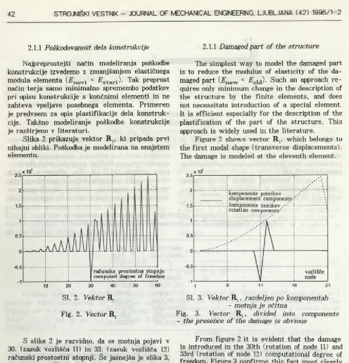
2.1.1 Poškodovanost dela konstrukcije 2.1.1 Damaged part of the structure
Najpreprostejši način modeliranja poškodbe konstrukcije izvedemo z zmanjšanjem elastičnega modula elementa ( Enovi < Eslari ). Tak preprost način terja samo minimalno spremembo podatkov pri opisu konstrukcije s končnimi elementi in ne zahteva vpeljave posebnega elementa. Primeren je predvsem za opis plastifikacije dela konstruk cije. Takšno modeliranje poškodbe konstrukcije je razširjeno v literaturi.
Slika 2 prikazuje vektor R lf ki pripada prvi nihajni obliki. Poškodba je modelirana na enajstem elementu.
Fig. 2. Vector Rt
The simplest way to model the damaged part is to reduce the modulus of elasticity of the da maged part (Enew < Eold). Such an approach re quires only minimum change in the description of the structure by the finite elements, and does not necessitate introduction of a special element. It is efficient especially for the description of the plastification of the part of the structure. This approach is widely used in the literature.
Figure 2 shows vector R lt which belongs to the first modal shape (transverse displacements). The damage is modeled at the eleventh element.
SI. 3. Vektor R ,, razdeljen po komponentah
- motnja je očitna
Fig. 3. Vector R j, divided into components
- the presence of the damage is obvious
S slike 2 je razvidno, da se motnja pojavi v 30. (zasuk vozlišča 11) in 33. (zasuk vozlišča 12) računski prostostni stopnji. Še jasnejša je slika 3, kjer je vektor R t razdeljen po posameznih kompo nentah. Ker prva nihajna oblika pripada prečnemu nihanju, so komponente vzdolžnih pomikov enake nič. S slike 3 je dalje razvidno, da komponente pomikov monotono naraščajo (izjema je zadnji element). Komponente zasukov dosežejo ekstremni vrednosti v vozliščih 11 in 12, torej v vozliščih, ki omejujeta element 11, kjer se sprememba togosti dejansko pojavi. Vektorji, ki pripadajo višjim ni hajnim oblikam, izkazujejo podobno obnašanje. Vrednosti pomikov so numerično večje, vendar ne omogočajo identifikacije motnje.
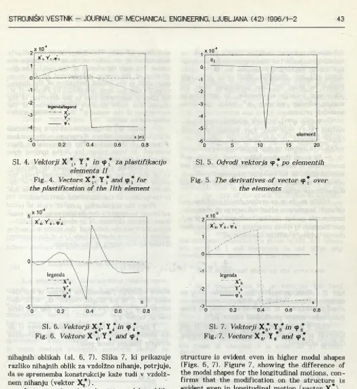
Slika 4 prikazuje vektorje X* in tp*. Vektor «p* jasno kaže vpliv spremembe konstruk cije: na plastificiranem elementu naredi vektor <pt preskok. Yuen 1111 ne analizira višjih nihajnih oblik, vendar trdi, da poškodbe dela konstrukcije v višjih nihajnih oblikah ni moč zaznati. Vendar je sprememba konstrukcije opazna tudi v višjih
From figure 2 it is evident that the damage is introduced in the 30th (rotation of node 11) and 33rd (rotation of node 12) computational degree of freedom. Figure 3 confirms this fact most clearly - vector R, is divided into components. Since the first modal shape belongs to the transverse mo tion, all components of longitudinal motions are equal to zero. From figure 3 it is further evident that the components of the displacements are monotonously increasing (the exception is the last element). The components of the rotations achieve their maximums at nodes 11 and 12. These are the nodes that bound the element 11, where the change of stiffness is actually modelled. The vec tors that belong to higher modal shapes exhibit similar behaviour. The values of the displacements are numerically higher but they do not allow for identification of the change.
Sl. 4. Vektorji X *, Y * in tp * za plastifikacijo elementa 11
Fig. 4. Vectors X* Y * and tp * for the plastification of the 11th element
X 1 ( V
SI. 6. Vektorji X * Y * in tp * Fig. 6. Vektors X *, Y * and «p *
nihajnih oblikah (sl. 6, 7). Slika 7, ki prikazuje razliko nihajnih oblik za vzdolžno nihanje, potrjuje, da se sprememba konstrukcije kaže tudi v vzdolž nem nihanju (vektor X*).
Jasno je vidno, da tudi višje modalne oblike kažejo lokacijo poškodovanega dela. V analizi, ki jo podajajo Pandey in drugi 161, so v računskem modelu upoštevani samo prečni pomiki brez zasu kov in vzdolžnih pomikov, lastni vektorji pred primerjavo nihajnih oblik niso normalizirani na lastno frekvenco, opazovana pa je absolutna vred nost vektorjev Y *. Za lociranje poškodb je upo rabljena aproksimacija drugih odvodov prečnih pomikov. Največja absolutna vrednost spremembe nihajne oblike naznačuje lokacijo spremembe na konstrukciji. Absolutne vrednosti razlik nihajnih oblik in aproksimacij odvodov zasukov sicer pou darijo lokacijo spremembe, vendar za račun z ab solutnimi vrednostmi ni fizikalne osnove.
S slik 4, 6 in 7 je razvidno, da je spremembo togosti mogoče locirati že s slike vektorjev tp*.
Sl. 5. Odvodi vektorja tp * po elementih
Fig. 5. The derivatives of vector tp* over the elements
X 6. Y 6 . <P 6
le g e n d a " ^ X ’6
n <P 6
--- X ■ 3--- •--- — --- ■
---0 0 .2 0 .4 0 .6 0 .8
SI. 7. Vektorji X* Y * in tp * Fig. 7. Vectors X* Y * and tp*
structure is evident even in higher modal shapes (Figs. 6, 7). Figure 7, showing the difference of the modal shapes for the longitudinal motions, con firms that the modification on the structure is evident even in longitudinal motion (vector X 6).
It is clearly evident that even higher modal shapes expose the location of the damaged part. In the analysis given by Pandey et al. (61 only trans verse displacements (neglecting longitudinal dis placements and rotations) are considered. Eigen vectors are not normalised by the eigenfrequency prior to the comparison of modal shapes, and only absolute values of vectors Y * are considered. To locate the damage the approximation of second de rivatives of transverse displacements is used. The maximum absolute difference of the modal sha pes’ change indicates the location of the damage
on the structure. The absolute values of the mo dal shapes’ differences emphasise the location of the change, but there is no physical interpretation for absolute values.
Spremembo namreč enolično določa preskok na mestu spremembe (ne samo sprememba predzna ka). Odvod vektorja «p* označen kot 0 , — ekvi valent drugemu odvodu pomikov, ki so ga vpeljali Pandey in drugi 161, ima pomembno vlogo pri odkrivanju lokacije spremembe. Za natančnejšo analizo odvodov vektorja «p * lahko uporabimo naslednje prijeme.
— Vektor «p * je mogoče aproksimirati s poli nomom (AM ) tega reda, kjer pomeni N število členov vektorja, in nato analizirati polinom. Pri večjih N ta metoda ne daje pričakovanih rezultatov-— Po vzoru Pandeya lahko odvod vektorja tp * izračunamo iz vektorja Y • , vendar se je treba pri tem zavedati, da ne moremo izračunati vrednosti odvoda v najmanj štirih točkah (zaradi postopka numeričnega odvajanja).
Izkaže se, da je za analizo dovolj približno iz računati konstanten odvod vektorja prek elementa. Izračunamo ga kot razliko vrednosti vektorja «p* med končnim i j+1 ) in začetnim ( j) vozliščem ele menta, deljeno z dolžino elementa ali:
of vectors «p* only. The change is in fact clearly determined by an interruption at the change lo cation (not only the change of the sign). The de rivative of the vector tp* denoted by 0 2- — an equivalent to the second derivative of the displa cements that has been introduced by Pandey et al. 161 plays a significant role in the detection of the change. For more accurate determination of the derivatives of the vector tp* the following appro aches can be used.
— Vector tp j is approximated by a polynomial of a (AM) degree, where N represents the number of terms of the vector. The polynomial is then analysed. At large values for A the method does not exhibit the expected results.
— Following the idea by Pandey the derivati ve of the vector tp* can be computed from the vector Y* (bearing in mind that the value of the derivative cannot be computed in four points due to the process of the numerical derivation).
From the engineering point of view it is sufficient to compute the derivative as being con stant over an element. It is computed as a diffe rence between the values of the vector tp2- in the ending (j +1) and starting node ( j ) of the element, divided by the length of the element:
kjer z j označujemo številko elementa, z lj pa njegovo dolžino. Vektor 0 J katerega elementi so
d(<p*j)/dx(j = 1. 2, ..., AM) ima torej en člen
manj kakor njegov predhodnik vektor tp * .
Sliki 5 in 8 jasno izkazujeta element 11 pri katerem se vrednost odvoda sunkovito spremeni (lokalni ekstrem).
Sl. 8. Odvod vektorja cp *
Fig. 8. Derivative of the vector cp*
where subscript j denotes the number of the ele ment and L is its length. Vector Qj w ith ele ments d j ) / d x {) = 1, 2, ..., AM) has one term less as vector tp*
Figures 5 and 8 clearly indicate element 11 as the element where the value of the derivative abruptly changes (local peak).
X 10'8
SI. 9. Primerjava vektorjev tp *
za različne globine razpok
Fig. 9. Comparison of vectors tp *
Za simuliranje razpoke uporabimo tudi po seben končni element za ravninske konzole pra vokotnega prereza [91 s prečno razpoko. Pred postavimo, da se velikost poškodbe s časom ne spreminja in poškodba vpliva samo na togostno matriko, ne pa tudi na masno. Uporaba takega elementa terja podatka o natančni lokaciji in globini razpoke.
Sklepi, ugotovljeni pri analizi zmanjšanja elastičnega modula, so potrjeni tudi tukaj. Veli kost vektorjev se zvečuje z globino razpoke. Slika 9 prikazuje vektorje tpj* za globine razpoke 1/10, 2/10, 3/10 in 4/10 višine prereza.
Globoke razpoke so zelo prilagodljive in se obnašajo bolj ali manj kot členki. V primeru ob ravnavane konzole se to kaže tako, da del desno od razpoke oscilira v približno enaki obliki kakor pri nepoškodovani konstrukciji, le z večjo ampli tudo. To je razvidno s slike 9, kjer so vrednosti desno od razpoke bolj ali manj linearne.
Faktorji KMU (MAC) in KMUK (COMAC) so za primer zmanjšanja togosti izračunani v študiji [61. Vse vrednosti so enake 1 in kot take ne dajejo nobene podlage za analizo spremembe.
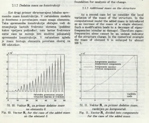
2.1.2 Dodatna masa na konstrukciji
Kot drugi primer obravnavajmo lokalno spre membo mase konstrukcije. V računskem modelu jo dosežemo s povečanjem mase enega elementa. Taka sprememba konstrukcije običajno vodi do zmanjšanja lastnih frekvenc sistema (podobno kakor vpeljava poškodbe), zato lastne frekvence same zase ne morejo biti enolični pokazatelj spremembe konstrukcije. V računskem zgledu je masa šestega elementa povečana skoraj za 100 odstotkov.
Sl. 10. Vektor R, za primer dodatne mase na elementu 6
Fig. 10. Vector R, for the case of the added mass on the element 6
For the simulation of the crack a special fi nite element for plane beams w ith a rectangular cross-section 191 w ith a uniform transverse crack was used. This model supposes that the crack depth remains constant w ith the time, and that the crack influences only the stiffness without affecting the mass matrix. The implementation of such an element requires data about the pre cise crack location and crack depth.
The conclusions obtained from the analysis with the reduction of the modulus of the elasti city are valid also for such a model of the dama ge. The amplitude of the vectors increases to gether with the crack depth. Figure 9 shows vectors <p* for crack depths 1/10, 2/10, 3/10 and 4/10 of the beam height.
Deep cracks are very flexible and they behave more or less as pins. In the cantilever under con sideration this is reflected in the fact that the part to the right of the crack oscillates in approxi mately equal shape as in the undamaged case. Only the amplitude of the oscillations is larger. This is clearly seen from the figure 9, where the values to the right of the crack are more or less linear.
MAC and COMAC factors for the case of the stiffness reduction are given in (6). All values are equal to 1 and therefore do not offer any foundation for analysis of the change.
2.1.2 Additional mass on the structure
As a second case let us consider the local variation of the mass of the structure. In the computational model the added mass is introduced as an increase of the mass of a single element. Such a modification leads to a decrease of eigen- frequencies (similar as damage). Therefore eigen- frequencies alone cannot be an unique indicator of the structure change. In the numerical example the mass of element 6 is enlarged by almost 100 %.
komponente | displacement komponente
r o t a t i o n comf
components asukov
vozlišče node
SI. 11. Vektor za primer dodatne mase, razdeljen po komponetah
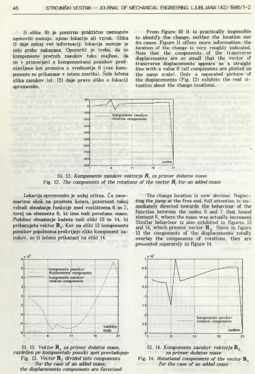
S slike 10 je ponovno praktično nemogoče ugotoviti motnjo, njeno lokacijo ali vzrok. Slika 11 daje nekaj več informacij: lokacija motnje je zelo grobo nakazana. Opozoriti je treba, da so komponente prečnih zasukov tako majhne, da so v primerjavi s komponentami pomikov pred stavljene kot premica z vrednostjo 0 (vse kom ponente so prikazane v istem merilu). Sele ločena slika zasukov (sl. 12) daje pravo sliko o lokaciji spremembe.
From figure 10 it is practically impossible to identify the change, neither the location nor its cause. Figure 11 offers more information: the location of the change is very roughly indicated. Note that the components of the transverse displacements are so small that the vector of transverse displacements appears as a straight line with a value 0 (all components are plotted on the same scale). Only a separated picture of the displacements (Fig. 12) exhibits the real si tuation about the change locations.
100 0
-100
-200
-300
-400
-500
-600
-700
-800
-900 1
komponente zasukov
vozlišče
SI. 12. Komponente zasukov vektorja R, za primer dodatne mase
Fig. 12. The components of the rotations of the vector R t for an added mass
Lokacija spremembe je sedaj očitna. Če zane marimo skok na prostem koncu, pozornost takoj vzbudi obnašanje funkcije med vozliščema 6 in 7, torej na elementu 6, ki ima tudi povečano maso. Podobno obnašanje kažeta tudi sliki 13 in 14, ki prikazujeta vektor R 2. Ker na sliki 13 komponente pomikov popolnoma prekrijejo sliko komponent za sukov, so ti ločeno prikazani na sliki 14.
The change location is now obvious. Neglec ting the jump at the free end, full attention is im mediately directed towards the behaviour of the function between the nodes 6 and 7 that bound element 6, where the mass was actually increased. Similar behaviour is also exhibited in figures 13 and 14, which present vector R 2. Since in figure 13 the components of the displacements totally overlay the components of rotations, they are presented separately in figure 14.
... ^Komponente pomikov ... . . : displacement components :
(rotation com] jonents
1 ** : node
1 6 11 16 21
X 10‘
SI. 13. Vektor R 2 za primer dodatne mase, razdeljen po komponetah; pomiki spet prevladujejo
Fig. 13. Vector R 2 divided into components for the case of an added mass; the displacements components are favorised
Sl. 14. Komponente zasukov vektorja R 2
za primer dodatne mase
Fig. 14. Rotational components of the vector R2
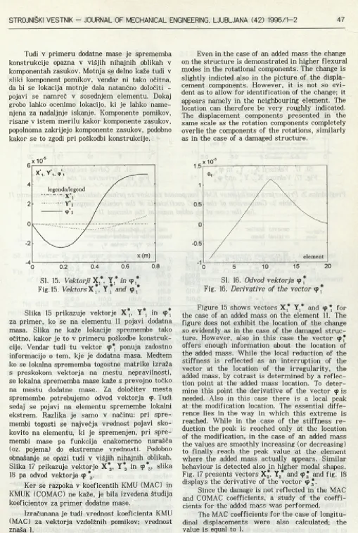
Tudi v primeru dodatne mase je sprememba konstrukcije opazna v višjih nihajnih oblikah v komponentah zasukov. Motnja se delno kaže tudi v sliki komponent pomikov, vendar ni tako očitna, da bi se lokacija motnje dala natančno določiti - pojavi se namreč v sosednjem elementu. Dokaj grobo lahko ocenimo lokacijo, ki je lahko name njena za nadaljnje iskanje. Komponente pomikov, risane v istem merilu kakor komponente zasukov, popolnoma zakrijejo komponente zasukov, podobno kakor se to zgodi pri poškodbi konstrukcije.
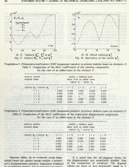
Slika 15 prikazuje vektorje X*, Y* in «p* za primer, ko se na elementu 11 pojavi dodatna masa. Slika ne kaže lokacije spremembe tako očitno, kakor je to v primeru poškodbe konstruk cije. Vendar tudi tu vektor cp* ponuja zadostno informacijo o tem, kje je dodatna masa. Medtem ko se lokalna sprememba togostne matrike izraža s preskokom vektorja na mestu nepravilnosti, se lokalna sprememba mase kaže s prevojno točko na mestu dodatne mase. Za določitev mesta spremembe potrebujemo odvod vektorja «p. Tudi sedaj se pojavi na elementu spremembe lokalni ekstrem. Razlika je samo v načinu: pri spre membi togosti se največja vrednost pojavi sko kovito na elementu, ki je spremenjen, pri spre membi mase pa funkcija enakomerno narašča (oz. pojema) do ekstremne vrednosti. Podobno obnašanje se opazi tudi v višjih nihajnih oblikah. Slika 17 prikazuje vektorje X*, Y* in cp 3, slika 18 pa odvod vektorja tp * .
Ker se razpoka v koeficentih KMU (MAC) in KMUK (COMAC) ne kaže, je bila izvedena študija koeficientov za primer dodatne mase.
Izračunana je tudi vrednost koeficienta KMU (MAC) za vektorja vzdolžnih pomikov; vrednost znaša 1.
Even in the case of an added mass the change on the structure is demonstrated in higher flexural modes in the rotational components. The change is slightly indicted also in the picture of the displa cement components. However, it is not so evi dent as to allow for identification of the change; it appears namely in the neighbouring element. The location can therefore be very roughly indicated. The displacement components presented in the same scale as the rotation components completely overlie the components of the rotations, similarly as in the case of a damaged structure.
Figure 15 shows vectors X* Y * and cp * for the case of an added mass on the element 11. The figure does not exhibit the location of the change so evidently as in the case of the damaged stru c ture. However, also in this case the vector cp* offers enough information about the location of the added mass. While the local reduction of the stiffness is reflected as an interruption of the vector at the location of the irregularity, the added mass, by cotrast is determined by a reflec tion point at the added mass location. To deter mine this point the derivative of the vector cp is needed. Also in this case there is a local peak at the modification location. The essential diffe rence lies in the way in which this extreme is reached. While in the case of the stiffness re duction the peak is reached only at the location of the modification, in the case of an added mass the values are smoothly increasing (or decreasing) to finally reach the peak value at the element where the added mass actually appears. Similar behaviour is detected also in higher modal shapes. Fig. 17 presents vectors X* Y3* and cp* and fig. 18 displays the derivative of the vector cp *.
Since the damage is not reflected in the MAC and COMAC coefficients, a study of the coeffi cients for the added mass was performed.
Preglednica 2: Primerjava koeficientov KMU komponent zasukov za primer dodatne mase na elementu 11
Table 2: Comparison of the MAC coefficients of the rotation components for the case of an added mass at the element 11
osnovni nosilec original beam
v e k to r Uj- v e c to r uj j = 1
i = 1 1,000
/ = 2 0,009
/ = 3 0,009
i = 4 0,010
i = 5 0,010
nosilec z dodatno maso beam with an added mass
vektor Vj - vector \j
j = 2 j = 3 j = 4 7 = 6
0,019 0,010 0,005 0,007
0,998 0,007 0,029 0,015
0,011 1 0,015 0,012
0,011 0,010 0,993 0.005
0,011 0,011 0,011 0,998
Preglednica 3: Primerjava koeficientov KMU komponent pomikov za primer dodatne mase na elementu 11
Table 3: Comparison of the MAC coefficients of the transverse displacement components for the case of an added mass at the element 11
osnovni nosilec nosilec z dodatno maso
original beam beam with an added mass
v e k to r Vj — v e c to r \ j
v e k to r u^--v e c to r Uj j= 1 j = 2 J = 3 7 = 4 7 = 6
i =1 1,000 0,396 0,060 0.095 0.033
i = 2 0,383 1,000 0,229 0,085 0.103
/ = 3 0,062 0,235 1 0.167 0,044
/ = 4 0,088 0.065 0,148 0,998 0.091
/ = 5 0,035 0,101 0,045 0,120 0,999
Opazimo lahko, da so vrednosti zunaj diago nalnih členov pri zasuku mnogo manjše v primer javi s komponentami pomikov, diagonalne vrednosti pa so praktično enake 1, kar ni primerno za ugotav
ljanje spremembe na konstrukciji. Vrednosti koe ficientov KMUK so bile izračunane v 20 vozliščih (razen v vpetem). Upoštevanih je šest nihajnih ob lik (L=6), ki pripadajo prečnemu nihanju. Izraču nane vrednosti so bile praktično enake 1 (vrednost, ki je najbolj odstopala je bila 0,99965104440336).
2.1.3 Oslabitve/okrepitve prereza
Obravnavane so bile tudi oslabitve in okre pitve prereza, kjer se pojavi hkrati sprememba togostne in masne matrike. Pojavijo se lahko kot rezultat proizvodnega procesa zaradi nenatančne izdelave konstrukcije, npr. kot povečanje oz. zmanjšanje prereza. Taka študija je torej zanimiva predvsem z vidika potrditve računskega modela.
2.1.3 The weakening/hardening of the cross-section
The weakening and hardening of the cross- sections were also considered. In such cases the change of stiffness occurs simultaneously with the variation of the mass matrix. They may be the result of a manufacturing process due to an impre cise production as a reduction or enlargement of the cross-section. Such a study is therefore inte resting mostly from the point of supervision and validation of the computational model chosen.
SI. 19. Vektor R t za primer povečanja prereza elementa 5; motnja je očitna
Fig. 19. Vector R, for the case of enlargement of the cross section at the element 5;
the disturbation is obvious
SI. 20. Komponente vektorja Rj ; komponenti zasukov in pomikov izkazujeta lokacijo motnje
Fig. 20. Components of the vector R ; ;
the components of the rotations and displacement exhibit the location of the disturbance
Na sliki 20 je motnja zelo očitna. Bistvena razlika med sliko 20 in drugimi slikami, ki prika zujejo vektorje R po komponentah, je, da tudi kom ponente pomikov na sliki 20 jasno (če ne celo jas neje) izkazujejo lokacijo motnje. Enaka težnja je opazna tudi pri vektorjih R, ki pripadajo preostalim višjim frekvencam. S slike 20 je tudi razvidno, da so komponente pomikov že bistveno večje od kom ponent, ki pripadajo zasukom.
Sl. 21. Vektorji X* Y * in ^ * za primer oslabitve prereza
Fig. 21. Vectors X*, Y * and «p * for reduction of the cross-section
The location of the disturbance from fig. 20 is evident. The essential difference between fig. 20 and other figures, presenting vectors R by their components, is that also the displacement compo nents clearly exhibit the location of the distur bance. The location is somehow even more evident from the displacement components than from the rotation components. The same stands for vectors R that belong to higher frequencies. It is also ap parent from figure 20 that the displacement com ponents are higher than the rotation components.
X 10'4
SI. 22. Vektorji X*, Y * in <p * primer okrepitve prereza
Slika 21 prikazuje drugi vektor za primer oslabitve prereza, slika 22 pa prikazuje prvi vektor za primer okrepitve prereza. Razvidno je, da je sprememba togostne matrike prevladujoča v pri merjavi s spremembo masne matrike, saj so re zultati podobni kakor pri spremembi togosti.
2.2 Drugi primer
Figure 21 shows the second vector for the reduction of the cross section, and figure 22 dis plays the first vector for the case of enlargement of the cross section. It is evident from both figu res that the change of the stiffness is dominant over the change of the mass. The results obtained are in fact similar to those obtained for the mo dification of the stiffness only.
2.2 Second example Prvi primer, dokaj preprost, je postregel s
kopico informacij, katerih splošno veljavnost je treba preveriti še na zapletenejših konstrukcijah. Kot drugi primer obravnavajmo konstrukcijo na sliki 23.
The first example, although simple, offered a considerable amount of information. The next example was used to verify the data on a more complex structure. As the second example the following structure was chosen (Fig. 23):
1 2 3 4 5 6 7 8 9 10 11 12 13 14
I N I I I I P
1 5 1 1 1 1 I I I
4.0 m 16 17 18 19 20
10.0 m
6.0 m E = 3,1010 N/m2 p = 2650 kg/m3
SI. 23. Drugi primer
Fig. 23. Second structure
izmere: elementi 1-4: b /h = 0,20/0,20 m -,
5-14: b /h = 0,20/0,30 m nosllec
15-20: b /h = 0,20/0,25 m steber
dimensions: elements 1-4: b /h = 0.20/0.20 m . orv, 5-14: b /h = 0.20/0.30 m beam 15-20: b /h = 0.20/0.25 m column
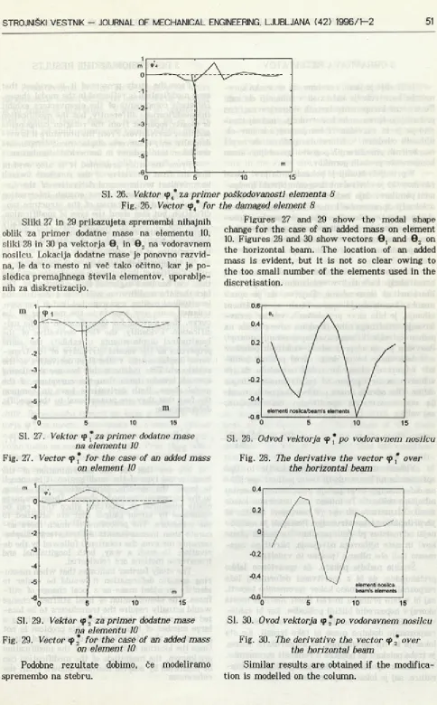
V prejšnjem podpoglavju se je izkazalo, da so vektorji cp * oziroma 0 ,- najzanesljivejši kazalec spremembe na konstrukciji, zato sedaj vektorji R;, X*, YJ; niso več prikazani. Slika 24 prikazuje vektor tpt za primer poškodovanosti elementa 8 (zmanjšanje elastičnega modula). Vektor je izrisan pravokotno na konstrukcijo (narisana s črtkano črto ) v povečanem merilu zaradi dvojnega merila. S slike 25, ki prikazuje odvod <p*, po nosilcu, je jasno razvidno, da prihaja do skoka na elementu 8 zaradi poškodbe. Motnja je opazna tudi v višjih nihajnih oblikah (sl. 26).
Sl. 24. Vektor cp * za primer poškodovanosti elementa 8
Fig. 24. Vector cp * for the case of damaged element 8
Previous studies showed that the vectors cp*
and 0 j are the most reliable indicators for the change on the structure, and therefore in this example the vectors Ry, X *and Y* are no longer considered. Figure 24 shows vector tp* for the case of damaged element 8 (reduced elasticity modulus). The vector values are plotted transversely to the main axis of the elements (indicated by a dashed line) in a multiplied scale due to the dual scale. From figure 25, showing the derivative of the vec tor cp*, over the beam, it is evident that there is interruption on element 8. This interruption re flects the damage at this element. The disturbance is also evident at higher modal shapes (Fig. 26).
SI. 25. Odvod vektorja zasukov po prečki
Sl. 26. Vektor <p* za primer poškodovanosti elementa 8
Fig. 26. Vector <p* for the damaged element 8
Sliki 27 in 29 prikazujeta spremembi nihajnih oblik za primer dodatne mase na elementu 10, sliki 28 in 30 pa vektorja 0 , in 0 2 na vodoravnem nosilcu. Lokacija dodatne mase je ponovno razvid na, le da to mesto ni več tako očitno, kar je po sledica premajhnega števila elementov, uporablje nih za diskretizacijo.
Figures 27 and 29 show the modal shape change for the case of an added mass on element 10. Figures 28 and 30 show vectors 0 , and 0 2 on the horizontal beam. The location of an added mass is evident, but it is not so clear owing to the too small number of the elements used in the discretisation.
SI. 27. Vektor tp * za primer dodatne mase na elementu IO
Fig. 27. Vector tp * for the case of an added mass on element 10
SI. 28. Odvod vektorja cp* po vodoravnem nosilcu
Fig. 28. The derivative the vector tp * over the horizontal beam
SI. 29. Vektor tp* za primer dodatne mase na elementu 10
Fig. 29. Vector tp * for the case of an added mass on element 10
Podobne rezultate dobimo, če modeliramo spremembo na stebru.
Sl. 30. Ovod vektorja tp * po vodoravnem nosilcu
Fig. 30. The derivative the vector cp * over the horizontal beam
3 OBRAVNAVA REZULTATOV
Iz študije je jasno razvidno, da se vsaka spre memba konstrukcije kaže tudi v nihajnih oblikah. Posamezne komponente lastnih vektorjev različno prikazujejo spremembo konstrukcije, najbolj izra zito pa je ta razvidna iz komponent zasukov oz. njihovih odvodov. V literaturi opazimo, da se pri numeričnih simuliranjih pogosto uporabljajo samo komponente prečnih pomikov.
V pričujoči študiji je pokazano, da prvi odvod zasukov (ki je ekvivalent drugemu odvodu kompo nent pomikov ) daje zadostne informacije ne samo o lokaciji spremembe konstrukcije, temveč je iz oblike mogoče sklepati o tipu spremembe. Spre memba mase, ki je v literaturi popolnoma zane marjena, se namreč v vektorju odvodov zasukov kaže popolnoma drugače kakor npr. variacija to gosti.
Nadalje se je izkazalo, da se sprememba konstrukcije kaže tudi v vzdolžnem nihanju, ki v literaturi ni obravnavano. Dejstvo, da je spre memba konstrukcije opazna tudi v vzdolžnem nihanju, je bilo sicer pričakovano, vendar obrav navanje vzdolžnega nihanja odpira nove poglede na pomen krivulje, ki omogoča razpoznavanje motnje. Razvidno je, da se prvi odvod vzdolžnih pomikov u obnaša enako kakor drugi odvod prečnih pomi kov v (prvi odvod zasukov), kar naznačuje, da gre v bistvu za širši pojem od zakrivljenosti nihajne oblike. Oba odvoda imata namreč skupno lastnost, da sta sorazmerna specifičnim deformacijam, saj velja:
_ 9_u _ d ( - y cp)
£ 3 X 3 X
Vidimo, da je za določitev lokacije in tipa spremembe na konstrukciji treba poznati specifič ne deformacije, ki pripadajo posameznim lastnim nihajnim oblikam. Te mnogo laže izmerimo kakor zasuke. Izmerimo jih npr. z merilnimi lističi, ki jih prilepimo na konstrukcijo. Postopek je natanč nejši od meritev prečnih pomikov ( in morda zasu kov) in nato njihovega odvajanja, hkrati pa zaja memo tudi obe nihanji (prečno in vzdolžno).
Študija nadalje pokaže, da upravičeno lahko pričakujemo, da bi z meritvami deformacij laže razpoznali dodatno maso kakor spremembo togosti, saj bi v tem primeru morali imeti merilna mesta skoraj v neposredni bližini poškodbe, kar bi zahte valo veliko število merilnih mest. Ta problem pri razpoznanju dodatne mase ni tako izrazit. Ko sta lokacija in tip spremembe na konstrukciji znana, je treba poiskati še podatke o velikosti spremembe. V ta namen uporabimo prilagojene postopke iz lite rature, saj je lokacija spremembe že znana.
3 DISCUSSION OF THE RESULTS
From the study presented it is evident that each modification is reflected in the modal shapes. Different components of the eigenvectors exhibit the modifications differently, but the modification is mostly apparent from the rotation components and their derivatives. From the literature it is evi dent that only transverse displacement components are taken into account in numerical simulations.
From the study presented it is also evident that the first derivative of the rotations (which is equivalent to the second derivative of the dis placement components) gives enough information not only about the location of the structure mo dification, but also about the type of modification. The change of the mass, which has been totally neglected in the existing literature, in fact ref lects completely differently than the damage — the variation of the stiffness.
It became further evident that the modifica tion is reflected in the longitudinal motions, and this, too, has been neglected in the literature. The fact that the modification will reflect itself in the longitudinal motion was expected, but it has con tributed some new aspects to the meaning of the curve, thus alowing for identification of the mo dification. Evidently, the first derivative of the longitudinal displacements u exhibits the same properties as the second derivative of the trans verse displacements v (the first derivative of the rotations). This indicates that we are discussing a much broader term than the curvature of the modal shape. Both derivatives have in common the fact that they are proportional to the specific deformations:
2
d X
We see that for the determination of the location and type of the modification it is enough to know the specific deformations that belong to the corresponding modal shapes. These are more easily measured as rotations since they can be measured by strain gauges that are attached to the structure. The procedure is much more ac curate than measurements of transverse displa cements (or even the rotations) followed by the de rivation. In such a way, both longitudinal and transverse motions are considered.
4 SKLEP
Predstavljena študija širše predstavlja vpliv spremenjene konstrukcije na lastne vektorje kakor je to znano iz literature. V analizi so upoštevani tudi vzdolžni (osni) pomiki, opazovan pa je vpliv različnih lokalnih sprememb konstrukcije. Prika zani rezultati potrjujejo, da se vse spremembe konstrukcije kažejo tudi v višjih nihajnih oblikah in ne samo v prvi nihajni obliki. Zaradi sistema tičnosti študije z uporabo različnih modifikacij je razvidno, da se različne spremembe različno ka žejo v posameznih nihajnih oblikah oziroma v po sameznih komponentah prostostnih stopenj. V idealnem primeru je moč iz oblike spremembe lastnih vektorjev določiti lokacijo in tip spre membe konstrukcije, za določitev njene amplitude pa so na voljo drugi postopki.
Upoštevanje osnih pomikov je pokazalo, da se določene zakonitosti poznajo tudi v nihajnih obli kah, ki pripadajo vzdolžnemu nihanju. Prav opa zovanje vpliva spremembe v vzdolžnem nihanju je pripeljalo do sklepa, da je za določanje mesta in tipa spremembe dovolj, če poznamo specifične deformacije, ki pripadajo lastnim nihajnim obli kam.
Rezultati so pokazali, da spremembe nihajnih oblik podajajo dovolj podatkov za določitev tipa in lokacije sprememb konstrukcije. Ločimo lahko dva osnovna primera: spremembo togostne matrike in spremembo masne matrike. Vsaka izmed njiju se drugače kaže v spremembi lastnih nihajnih oblik. Sprememba togosti se kaže s skokom vek torja cp * na mestu spremembe in z ostrim vrhom v sliki odvodov. Sprememba mase se izraža s pre vojno točko na mestu spremembe. Prav tako lahko trdimo, da je sprememba togostne matrike prevla dujoča nad spremembo masne matrike, saj pri kombinaciji obeh sprememb postane očitna samo sprememba togosti. Prikazani rezultati in podani sklepi veljajo za spremembo poljubne točke konstrukcije, vendar je treba za prikaz njihove veljavnosti v bližini vpetih delov konstrukcije uporabiti gostejšo diskretizacijo.
4 CONCLUSION
The study presented offers a wide illustra tion of the influence of structure modification on eigenvectors. In the analysis longitudinal (axial) displacements are also included, and the influence of several types of modification is investigated. The results obtained confirm the fact that all modifications reflect in all modal shapes, and not only in the first one. The systematisation of the study confirms that different modifications re flect differently in modal shapes or components of displacements (degrees of freedom). In the ideal case it is possible to determine the location and the type of modification from the eigen vectors change. For identification of the magni tude of the modification some other methods are known.
Consideration of the axial (longitudinal) dis placements showed that the principles are valid also for longitudinal motion. In fact, monitoring the modification change in the axial motion leads to the conclusion that specific deformations are needed for identification.
5 LITERATURA 5 REFERENCES
(11 Baruh, H.-Ratan, S.: Damage Detection in Flexible Structures, Journal of Sound and Vibrations, 166/1, 1993, 21-30.
(2) Bohte, Z.: Numerične metode. Zveza organizacij za tehnično kulturo Slovenije. Ljubljana. 1987.
13) Cawley P.-Adams, R.D.: The Location of De fects in Structures from Measurements of Natural Fre quencies. Journal of Strain Analysis, Voi. 14, 1979/2.
141 Choy, F.K.-Liang, R.-Xu, P.: Fault Identifica tion of Beams on Elastic Foundation. Computers and Geotechnics 17, 1995, 157-176.
151 Dimarogonas, A.D.: Modeling Damaged Structural Members for Vibration Analysis. Journal of Sound and Vibration, 112, 1987, 541-543.
161 Pandey, A.K.-Biswas, M.-Samman, M.M.: Da mage Detection from Changes in Curvature Mode Shapes. Journal of Sound and Vibration, 145/2, 1991, 321-332.
171 Salawu, O.S.-Williams, C.: Bridge Assessment Using Forced-Vibration Testing. Journal of Structural Engineering. Voi. 121/2, February, 1995.
181 Singh, R.K.-Smith, H.A.: Comparison of Com putational Effectiveness of the Finite Element Formula tion in Free Vibration Analyses. Computers & Structures, Voi.51, 1994/4., 381-391.
191 Skrinar, M.-Umek, A.: Ravninski linijski kon čni element nosilca z razpoko. Gradbeni vestnik, Ljublja na, 1996/1-2.
1101 Wood, W.L.: Note on Finite Element Predic tions of Natural Frequencies. Communications in Nume rical Methods in Engineering, Voi. 10. 1994, 731-734.
[Ill Yuen, M.M.F.: A Numerical Study of the Eigen- parameters of a Damaged Cantilever. Journal of Sound and Vibration 103/3, 1985, 301-310.
(121 12. PC-M atlab, Version 3.5. The MathWorks, Inc. 1984-1989.
1131 Fajfar, P.: Dinamika gradbenih konstrukcij. Univerza v Ljubljani, 1984.
Avtorjev naslov: mag Matjaž Skrinar, dipl. inž. Author’s Address: Mag. Matjaž Skrinar, Dipl. Ing.
Fakulteta za gradbeništvo Univerze v Mariboru Smetanova 17 2000 Maribor
Faculty of Civil Engineering University of Maribor Smetanova 17
2000 Maribor, Slovenia
Prejeto: 7_g_lgg5 Sprejeto:
Accepted:• 29.2.1996