in the population sciences published by the Max Planck Institute for Demographic Research Konrad-Zuse Str. 1, D-18057 Rostock · GERMANY www.demographic-research.org
DEMOGRAPHIC RESEARCH
VOLUME 21, ARTICLE 24 PAGES 719-758
PUBLISHED 10 NOVEMBER 2009
http://www.demographic-research.org/Volumes/Vol21/24/ DOI: 10.4054/DemRes.2009.21.24
Research Article
When Harry left Sally: A New Estimate of
Marital Disruption in the U.S., 1860 – 1948
Tomas Cvrcek
© 2009 Tomas Cvrcek.
This open-access work is published under the terms of the Creative Commons Attribution NonCommercial License 2.0 Germany, which permits use, reproduction & distribution in any medium for non-commercial purposes, provided the original author(s) and source are given credit.
1 Introduction 720
2 Direct historical evidence on marital disruption 721
3 The method of estimation 722
4 Data and adjustments 724
4.1 Size of marital cohorts 724
4.2 Intact marriages at τcensus 726
4.3 Incidence of widowhood 730
4.4 Duration profile of marital disruption 734
4.5 Assumptions – A Summary 736
5 Results and sensitivity 737
6 Further conceptual issues 749
7 Conclusion 751
8 Acknowledgements 752
When Harry left Sally:
A New Estimate of Marital Disruption in the U.S., 1860 – 1948
Tomas Cvrcek1
Abstract
The divorce rate is a poor indicator of marital instability because many marital disruptions never become divorces. This paper provides the first estimate of the rate of marital disruption in the U.S. in 1860 – 1948. In the long run, the cohort rate of marital disruption increased from about 10% in the mid-1860s to about 30% in the 1940s. Marital disruption rate was similar to the divorce rate after the Civil War but the two rates diverged wildly in the early 20th century. In 1900 – 1930, the disruption rate was
as much as double the divorce rate, implying that perhaps half of all disruptions never reached the court.
1. Introduction
Divorce and widowhood are two relatively public ways that a marriage can end. For a long time in American history, they have been subject to at least some level of public record keeping – even if the accuracy of the resulting statistics has been debated (U.S. Bureau of Census 1909:6; Reiss 1976:308; Haines 1998, 2006). Overwhelming historical evidence suggests, however, that many marriages ended long before the coroner or the divorce judge became involved2 and that frequently, both parties had
their reasons to keep silent about their marital disruption (Porter Benson 2007; Schwartzberg 2004, 2007).3 The general recognition among social scientists that a large
number of failed marriages passed “under the legal radar” is accompanied by an equally widespread skepticism about the retrievability of any reliable estimate of the actual rate of marital disruption (Brandt 1972:10; Crosby 1980:54; Eubank 1916:22; Plateris 1973:15; Price-Bonham and Balswick 1980:966; Igra 2007:75). Without a more precise idea about the prevalence of desertion and separation, the analysis of many aspects of marriage is left incomplete. The greater the number of desertions and separations that never achieved divorce status, the less reliable current divorce statistics are as a gauge of overall marital instability. Thus an estimate of the rate of marital disruption inclusive of desertion and separation is a critical research question.
This paper offers just such an estimate. My cohort-specific rates capture the proportion of each marriage cohort from 1860 to 1948 that ended in eventual disruption – whether through actual divorce, through mutually agreed separation, or through the unilateral “poor man’s divorce”, i.e. desertion and abandonment. From the cohort-specific proportions, I also impute annual rates of disruption and compare them to annual rates of divorce. The main conclusions emerging from this estimation are that the marital disruption rate was relatively close to the divorce rate immediately following the Civil War, but that the two rates wildly diverged in the early 20th century
until the Great Depression. Throughout the 1910s and 1920s, the disruption rate was as much as double the divorce rate, implying that perhaps half of all marital disruptions during this time never reached the court. The two rates then converged again by the time the Second World War broke out. The long-run trend of the cohort rate of marital disruption was to increase from about 10% in the mid-1860s to about 30% in the 1940s. The estimates are constructed using data on mortality, size and age composition of
2 Such evidence includes case files of the National Desertion Bureau of New York, established in 1911 (Igra 2007), claims of “contesting widows” for deceased husbands’ pensions from the Union Veterans records (Schwartzberg 2004), court records from cases prosecuting bigamy, or studies conducted by local charities in numerous American cities.
individual marriage cohorts, and on information, obtainable from the censuses of 1900, 1910 and 1950, regarding the survival of marriages from each marriage cohort – all demographic variables. No economic or social variables are directly used in the estimation. Whatever sensitivity the disruption estimates may have with respect to such variables, is not a product of the estimation methodology but rather a reflection of actual influence that economy and society had on the success of individual marriages.
2. Direct historical evidence on marital disruption
The two main sources regarding marital instability between 1860 and 1948 were charity studies4 and official divorce statistics (U.S. Bureau of Census 1909). Both are useful in
providing general stylized facts but as sources of reliable data, they are piecemeal and ridden with problems. The charity research consisted of isolated city-specific studies based on the cases of deserted women seeking aid. Their samples were unrepresentative due to self-selection (they included only aid seekers) and provided only a snapshot of the problem at one point in time. Yet in many aspects they all presented similar picture: incidence of desertions declined with duration of marriage (Brandt 1972; Marquis 1916; Zunser 1929), husbands overwhelmingly were the deserting party (Eubank 1916:14; Zunser 1929:101), and the most frequently cited immediate causes of desertion were the pregnant wife’s confinement (Smith 1901:4; Brandt 1972:35), a quarrel (Marquis 1916) and the husband’s drinking binge (Zunser 1929:103; Brandt 1972:35).
Desertion also appears in published divorce statistics. Divorce proceedings were fault-based throughout the relevant period.5 ‘Desertion and abandonment’ was the most
cited primary ground of divorce, accounting for about 40% of all divorce cases between 1867 and 1906 (U.S. Bureau of Census 1909:Table 22). Its share declined to about 17% by 1950 (Jacobson 1959:Table A25). However, it was also the most frequently abused legal ground for divorce, particularly by colluding spouses who hoped to secure a divorce decree at a time when courts were most unsympathetic to a mutually-agreed divorce (Eubank 1916; Britton 1916). Even those divorces that were rightfully granted for desertion and abandonment were only a belated legal recognition of a marital disruption that had occurred several years earlier because many states had statutory
4 See, for example, Smith (1901) for Boston, Britton (1916) for Cook County (Chicago), Marquis (1916) for Kansas City, Zunser (1929) for New York City. Brandt (1972) works with data provided by charities from several cities. Eubank (1916) is a meta-study of much of the city-specific research.
provisions that the abandonment had to last two to five years before it was admissible as a legal ground for divorce.6 Divorce was also costly in terms of time, money and
prestige and so the poorer strata of the society often resorted to simple desertion and abandonment – the “poor man’s divorce” – which often went unrecorded (Crosby 1980:53).7 Thus, historical divorce statistics are inaccurate and insufficient indicators of
the overall level of marital instability. Not only do they probably capture just a limited portion of all failed marriages, they also record the disruption with a delay, introduced by the slow operation of the courts (Plateris 1973:Table 16).
3. The method of estimation
Given how unreliable and incomplete the direct sources can be, I propose to estimate the disruption rate indirectly, by way of an accounting exercise. At any moment in time, a marriage must be in one of three states; (1) intact (2) terminated through death of one of the spouses (widowhood), or (3) ended through desertion, separation or divorce (disruption).8 If we have a good estimate, at some point in time, of the proportion of a
marriage cohort falling into two of the three states, we can infer the proportion falling into the third.
Figure 1 provides a stylized depiction of the lifetime experience of a marriage cohort of size M, married at time τ = 0. As time goes on, death and disruption take their toll until at τ* the cohort of marriages becomes extinct. Over the whole cohort lifetime, a proportion ω of these marriages end in widowhood while a proportion π ends in disruption. The relative size of these two proportions will depend on the time profiles of the competing risks of widowhood and disruption.9
6 Rhode Island was the state that required a desertion of five years as admissible grounds for divorce. The statute also stated, however, that the court had the discretion to grant divorce for shorter desertions (U.S. Bureau of Census 1909:317–318).
7 In his dissertation on desertion, Eubank (1916:22) summarized the motivation for silence among deserted women thus: “Except in occasional instance we have no way of getting information regarding deserted women who, for various reasons, may desire to refrain from making public record of having been forsaken: wives who, because of the disgrace of it, are not willing to have their status known; wives who, because of the fear of reprisals on the recreant husbands, do not dare to resort to legal means to bring them to task; wives who maintain silence because of preferring their absence to their presence; wives who for very loyalty to the disloyal absent ones shield them by not speaking; wives who would report their case if they only knew how to go about the perplexing business. How many of these there are and how their numbers might swell, we have no means of knowing.”
Figure 1: Widowhood and disruption in the lifetime of a marriage cohort
The fraction of disrupted marriages, π, is the indicator of interest. Its estimation requires combining data from several sources. As the diagram illustrates, the four crucial pieces of evidence used in estimation are (i) the initial size of marriage cohort,
M, (ii) the size of the marriage cohort still intact at some time later, such as at τcensus,
(iii) the age/time profile of the risk of widowhood and (iv) the duration profile of the risk of disruption. As it happens, all such information is available or can be reasonably estimated for the period from 1860 to 1948.
Estimation of the cohort rates of disruption is an iterative process starting from a naïve estimate of π0 = 0 (i.e. the first guess is that no marriages were disrupted and all
marriage dissolutions can be accounted for by death of one of the spouses). This iterative process can be summarized by the following equation:
(
)
⎥ ⎦ ⎤ ⎢ ⎣ ⎡ − − − + =∏
= − − T t i t ii A f t
T
F 1
1
1 1 ( ) ( )
) (
1 ω π α
π
π . (1)
Here, πi is the estimated proportion ever disrupted in the i-th iteration; ωt is the
mortality of a marriage cohort in year t of the cohort’s marriage and it is dependent on the marriage cohort’s age structure A; f(t) is the estimated proportion of lifetime
Duration τ M
Mπ
Marriage cohort size
terminated in disruption
αM: still intact
at τcensus Mω
terminated in death
τ*
disruptions occurring to the marriage cohort in the year t; F(T) is the cumulative proportion of lifetime disruptions occurring to the marriage cohorts in all years up to T; and α is the fraction of the marriage cohort still intact at the time of census which occurs in year T of the cohort’s married life. In other words, in the first iteration, a marriage cohort is simply “survived” (given that π0 = 0, then f(t) π0 = 0, i.e. no marriage
is disrupted under this naïve initial assumption), using the relevant mortality rates and age composition, between the year of marriage and the census date.The resulting imputed proportion of marriages still remaining is compared to α, which is the actual proportion of intact marriages observed in the census. The difference between the two, the marriages neither present in the census nor accounted for by the incidence of widowhood, is the expression in the square brackets and it is used to update πi for the
next iteration. The iteration converges when πi is large enough that the term inside
square brackets is zero.
The estimation process requires some specification of how marital disruption depends on the duration of marriage because, at the moment of census, each marriage cohort is captured at a different point along a timeline. With the exception of the very oldest marriages, any given number of intact marriages at the moment of census can be expected to contain some non-zero proportion of couples destined for disruption after the census. The duration profile (captured in equation (1) by f(t) and F(T)10) allows the
conversion of a snapshot of the incidence of disruption up to the moment of census into an estimate of a life-time percentage disrupted, π. For example, if the duration profile of disruption risk specifies that 75% of all of a cohort’s lifetime disruptions occur before the eleventh year of marriage (i.e. F(11) = 0.75) and the computations show that, as of 1950, 11.6% of all 1939 marriages have been disrupted, then one can estimate that a total of 15.47% (= 11.6/0.75) of all 1939 marriages will end up in disruptions over the life cycle of the marriage cohort.
4. Data and adjustments
4.1 Size of marital cohorts
The size of each marital cohort was obtained from Jacobson (1959: Table 2). The same data are also cited in Plateris (1973: Table 1). Jacobson (1959) obtained the number of marriages for 1867 – 1956 from National Office of Vital Statistics and estimated those for 1860 – 1866 himself. These numbers are the estimated annual totals of marriages solemnized on American soil.
Three issues need to be addressed. One is the reliability of these estimates. Jacobson (1959:9) himself describes the marriage recording in late 19th century to have
been in “wretched condition”. Both government reports that were commissioned (in 1887 and 1907) to investigate the state of American marriage and divorce concluded that the reporting was incomplete (U.S. Bureau of Census 1909, Vol I: 4). The totals published in the first report covered about two thirds of all counties, in the second report about 90% of all counties (Jacobson 1959:10). A continuous series of estimated annual number of marriages was then published in 1946 (these are the data used here).11
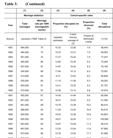
For the period 1887 – 1906, the 1946 estimates were about 5% higher than the yearly totals in the 1909 report and were reported rounded to thousands. Clearly, the National Office of Vital Statistics in 1946 adjusted and refined the original tallies collected for the 1909 report. For the post-1906 period, the numbers are no longer rounded (see Table 3, col. 1). If the extent of rounding is any measure, these numbers are precise enough for our purposes: the marriage totals are on the order of hundreds of thousand and millions (from 1912 onwards), so even an error of ten thousand marriages one way or other would not change the disruption estimates by more than one percentage point.
Jacobson (1959:Table 1) performed a simple accounting exercise to check the internal consistency of various data sources: he took the census totals for each marital status from two neighboring censuses and accounted for all possible flows in and out of a given marital status using government-collected data on marriage, migration, divorce and death. It turns out that for the transition from singlehood to marriage, the census statistics and the vital statistics are remarkably consistent, indicating either that they are relatively reliable or that their errors are so perfectly correlated as to cancel out. This latter proposition is highly improbable.
The second issue is the issue of common-law marriage. Even if the published data accurately capture the number of formal marriages, there could be a non-negligible proportion of couples who never legally formalized their marriage (thus absenting themselves from the annual totals) but still reported themselves as married in the census. The proportion of intact marriages would then be overestimated. It is unclear, however, how prevalent common-law marriage was. Shaw (1977:580) states that common law marriages had been “a historical necessity, since the desire to start a family would otherwise have been thwarted in scattered and isolated agricultural and mountain communities with difficult access to ministers or justices of the peace.“ With increasing urbanization and improved means of communications in the second half of the 19th century, the need for common-law marriage would be expected to decline. Moreover, common-law marriage had one important disadvantage compared to a formal marriage: it was not officially recorded, thus putting any legal claims arising out of such marriage (e.g. inheritance claims) at risk. A simple cost-benefit analysis
suggests that economic and social trends were working against common-law marriage. Developments in marriage law were acting in that direction also; Hall (1930:11) and Shaw (1977:585) show that more and more states were withdrawing legal validity from common-law marriage, passing laws which explicitly recognized only marriages performed by authorized persons and recorded by the locality as valid. Finally, Jacobson’s (1959: Table 1) accounting leaves little room for a high incidence of common-law marriage.12
All these arguments point to the conclusion that common law marriage was not very frequent, that it was limited to isolated communities or the poor (who had little chance of claiming property on the basis of marriage) and that it was in decline. Still, they did exist to some (unknown) extent and since I have no way of accurately accounting for them, my estimates of ατ, the proportion of marriages that were intact,
will be too high and my estimates of marital disruptions too low. Common law marriage therefore makes my estimates conservative.
The third issue is foreign marriages. Since the available data comprise only marriages solemnized on American soil, they can tell us nothing about the marriages of immigrants who already came to USA married. The problem is similar to that of a common-law marriage: the couple would be absent from the annual totals but appear as married in the census. Again, the proportion of intact couples would thus be overestimated. I deal with this problem in the following section.
4.2 Intact marriages at τcensus
The proportion of a marriage cohort that is still intact at a point in time is estimated with the aid of the IPUMS (Ruggles et al. 2008) and the totals from Jacobson (1959). Three US censuses – those in 1900, 1910 and 1950 – included a question about duration of current marriage (variable DURMARR).13 In all three instances, enumerators were
asked to record completed years of marriage.14 Based on the reported duration of
marriage, one can assign each marriage recorded in the census to a specific marriage cohort.
A few issues of definition and delimitation need to be addressed, however. One is the distinction between “native” marriage (that is, one solemnized on American soil)
12 Section 5 of this paper, nevertheless, discusses how the estimation results would be affected given various assumptions about the incidence of common-law marriage.
13 The 1950 census asked the question only of sample-line respondents.
and “foreign” marriage. I exclude foreign marriages because α, the proportion of intact marriages at τcensus, is calculated using Jacobson’s estimates of native marriages. I
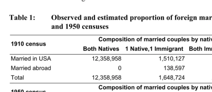
consider a marriage to be foreign if the reported duration of marriage is strictly greater than the reported years in the United States (variable YRSUSA1) of one of the spouses. Such foreign marriages amounted to about 6-7% of all marriages in 1900 and 1910. In the census of 1950, however, distinguishing between native and foreign marriages is not possible because the variable YRSUSA1 is not available. Still, given that immigration was relatively low from the 1920s onwards, it is probable that this is only a minor problem. Table 1 illustrates why. The top panel of Table 1 provides a decomposition of all marriages reported as intact in the 1910 census by nativity of spouses and place of wedding. The bottom panel of the table shows what such composition would look like for the marriages of the 1950 census, had the proportion of native and foreign marriages been the same as they had been in 1910, at the peak of immigration. From the left-most column, one can see that under such scenario, foreign marriages would comprise about 3% of all marriages (=1.1 mil/35.6 mil.). However, even such a percentage is likely a very high upper bound because a large fraction of those respondents in the 1950 census whose birthplace was outside the US had, in fact, come to the United States as children around the turn of the century and therefore got married in the US. In other words, most foreign marriages in the 1900 and 1910 censuses were marriages of immigrating families and since immigration was low throughout the interwar period, it is unlikely that the foreign marriages constituted a large share of total marriages in the 1950 census. The actual proportion of foreign marriages among all marriages in the 1950 census was therefore probably far below 3% and so they affect the overall calculations very little. Moreover, the little effect they have is to overestimate the proportion intact and underestimate the proportion disrupted, making the estimates, again, relatively conservative.
Another, even more complex, issue is to determine more precisely which marriages are truly intact. The marital status variable (MARST) distinguishes between respondents who were “married, spouse present” and those who were “married, spouse absent”. The latter is an imputed value assigned to those who reported themselves to be “married” but for whom a statistical program could not locate a spouse in their household. To what extent can a spouse alone be considered to live in an intact marriage? The absence of a husband or wife can be due to many things – seasonal employment, incarceration, attendance at a far-away college – none of which need to imply that the marital bonds have been broken. However, one could also be “married, spouse absent” as a result of desertion and abandonment. There is no clear-cut line between the two cases.15 The truth probably lies somewhere in-between: some but not
all “married, spouse absent” respondents were probably already deserted but were unaware of their unfortunate predicament. I provide separate estimate for either measure of intact marriage and discuss this issue further in section 5.
Table 1: Observed and estimated proportion of foreign marriages in the 1910 and 1950 censuses
Composition of married couples by nativity 1910 census
Both Natives 1 Native,1 Immigrant Both Immigrants Total
Married in USA 12,358,958 1,510,127 1,815,029 15,684,114 Married abroad 0 138,597 1,075,207 1,213,804
Total 12,358,958 1,648,724 2,890,236 16,897,918
Composition of married couples by nativity 1950 census
Both Natives 1 Native,1 Immigrant Both Immigrants Total
Married in USA (imputed) 30,734,789 2,340,730 1,477,067 34,552,585 Married abroad (imputed) 0 214,828 875,001 1,089,830 Total (observed) 30,734,789 2,555,558 2,352,068 35,642,415
Note: The tabulation for the 1910 census is based on both spouses’ birthplace (BPL) and the comparison between the duration of marriage (DURMARR) and the number of years they have lived in USA (YRSUSA1). If DURMARR ≤ min(YRSUSA1wife, YRSUSA1husband), a marriage is considered to have been solemnized in USA. The numbers for 1950 census show how many marriages would be foreign and how many American if the proportions in individual composition groups were the same as they had been in 1910.
The precision with which duration of marital status was recorded varied from census to census. The exact date of the census is important in interpreting data. The 1900 census was taken as of 1st June, the 1910 census as of 15th April and the 1950
census as of 1st April. In all three instances, the enumerators were instructed to record
full completed years of duration. Strictly speaking, a person who reported to have been married for, say, 16 years in the 1900 census would be expected to have married some time between 1st June 1883 and 31st May 1884. Consequently, it is not clear a priori
whether this marriage falls into the marital cohort of 1883 or 1884. A further complication is that the recall error probably increased with age of the respondents and duration of marriage. Plotting the totals of married population against marital duration revealed considerable heaping at multiples of five – especially for couples who had
been married for more than a decade. To correct for both problems, I assign 7/12 of the marital cohort to year 1883 and 5/12 to year 1884 and I smooth the resulting series using a 5-year centered moving average. Similar approach is applied to data from the 1910 and 1950 censuses with a view to the precise date of each census.
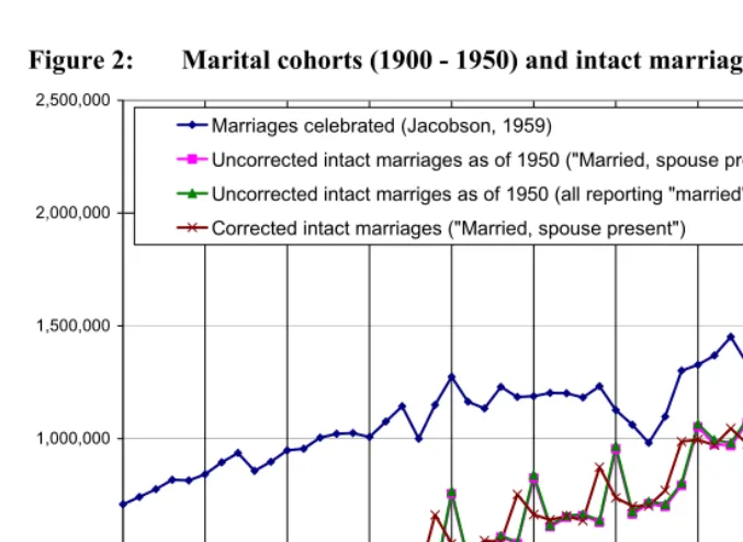
One exception to this correction is the 1940s. In Figure 2, total marriages display considerable variation during this decade. Plotted are also two measures of intact marriages surviving to the 1950 census where each marriage was assigned to a marriage cohort without any correction (i.e. the year of marriage was calculated as 1950 – DURMARR). The downswing in Jacobson’s estimates from 1942 to 1944, the explosion of 1944-46 and another decline in 1946-49 is clearly reproduced in the census data. Applying the specified correction for the date of the census (1st April 1950), i.e.
lagging three quarters of each marriage cohort by one year, would actually produce nonsensical results for the 1940s: for example, the number of 1945 marriages still intact in 1950 would then be higher than the total marriages solemnized in 1945. Thus, for the period 1942 – 1948 I retain the uncorrected census results. It is possible that the respondents’ recall for these marriages was better than at other times because they were closely tied to other important events in their lives, such as military enlistment (or leave) during the Second World War.
Note, however, how different the situation is for the 1930s. Jacobson’s estimates reach a trough in 1932, followed by a sharp upswing to 1934 and further growth until, in 1938, marriages decline again. This development, too, finds a counterpart in the census data – but misaligned by one year: the uncorrected intact marriages bottom out in 1933, the sharp upswing ends in 1935 and the latter decline occurs in 1939. Here, correcting for the fact that the 1950 census was taken as of 1st April and that therefore
about three quarters of intact marriages have to be lagged by one year produces the proper alignment.
Finally, couples who had only recently married (under 3 years) seem to be very deficient in reporting their marital duration, so in my estimation, I omit cohorts married within two years of the census.16
Figure 2: Marital cohorts (1900 - 1950) and intact marriages as of 1950
0 500,000 1,000,000 1,500,000 2,000,000 2,500,000
1900 1905 1910 1915 1920 1925 1930 1935 1940 1945 1950
Marriages celebrated (Jacobson, 1959)
Uncorrected intact marriages as of 1950 ("Married, spouse present") Uncorrected intact marriges as of 1950 (all reporting "married") Corrected intact marriages ("Married, spouse present")
Source: IPUMS, Jacobson (1959)
4.3 Incidence of widowhood
I exploit the age information in IPUMS to reconstruct the age distribution of wives and husbands in each marital cohort.17 Using sixteen 5-year age bins (from 10-14 years to
85+ years of age), I split each marriage cohort into 16x16 cells on the basis of husband’s and wife’s age. This allows me to pay relatively close attention to the age of spouses, when applying the mortality rates.
The incidence of widowhood was estimated from the available information on mortality during the period in question. Age-specific death rates by sex for 5-year age intervals come from Historical Statistics of the United States (Carter et al. 2006: Ab988–1047) for each year from 1900 onwards. These were converted into mortality rates (probabilities of death) using the relevant formula from Siegel and Swanson
(2004:289) where Da and Pa stand for number of deaths and for surviving population
and q represents mortality:
a a
a y
x y
D P
D q
5 2 1 5 1
5 = +
+ . (2)
From these, the probability was calculated of a marriage ending in widowhood in a given year, given the age of wife and of husband.
For the period 1860 – 1900, I used data from the U.S. mortality model presented in Haines (1998). Haines’ 5-year life tables, separate for men and women, are available at decadal intervals so the years between decades had to be interpolated. In order to capture the year-to-year variation in mortality, I applied the fluctuations in Massachusetts infant mortality (Carter et al. 2006:Ab 928) to the decadal trend in mortality in Haines’ life tables.18 Since the age categories in these life tables do not
extend beyond 75-79 years, I calculated the mortality for 80-84 year-olds and 85+ year olds on the assumption that the ratios between mortalities of these three age groups are roughly constant.19 Still, the death rates of these old age groups have very little effect
on overall estimation since only very few couples – even in the oldest marriage cohorts – fall into these age groups.
Adjustment needs to be made for the mortality differential between married men and women and the general population. Information on the mortality premium can be obtained from Willcox (1933:109) for the period 1924 – 1928 and from Grove and Hetzel (1968: Table 57) for 1940, 1950 and 1960. The published volumes for the 1890 and 1900 census also contain some information about death rates by marital status but these data mostly predate proper death registration and their reliability is often questioned (Haines 2006). By and large, however, the mortality differentials emerging from the 1890 – 1900 census death rates correspond with the mortality differentials observed in Grove and Hetzel (1968) (see Table 2). In order to adjust the general mortality risk for the mortality premium accruing to married men and women I therefore apply the 1890 premium to death rates in 1860 – 1890, the 1900 values to death rates in years 1900 – 1910, the 1924-28 values for the period 1920-1930 and I interpolate in the remaining periods.
18 Using infant mortality to proxy for movements in adult mortality hinges on how well the two are correlated. A simple correlation of death rates for infants and for 5-year age groups of men (from ages 10-14 to ages 80-84) ranges from 0.6 to 0.92; for women such correlation ranges from 0.74 to 0.93. If the death rates are de-trended (so that we measure only the correlation between fluctuations of death rates), the correlation coefficients fall to (0.33; 0.70) for men and (0.34; 0.58) for women.
Table 2: Ratios of death rates of married men and women to the death rates of all men and women
Males
Age <15 15-19 20-24 25-29 30-34 35-39 40-44 45-49 50-54 55-59 60-64 65-69 70-74 75+
1890 2.84 0.99 0.74 0.80 0.83 0.85 0.79
1900 1.61 0.68 0.70 0.79 0.84 0.87 0.80
1924-28 1.26 0.81 0.78 0.80 0.79 0.81 0.83 0.84 0.86 0.87 0.88 0.89 0.85
1940 0.56 0.81 0.76 0.81 0.85 0.86 0.88 0.88 0.89 0.83
1950 0.52 0.74 0.77 0.84 0.87 0.89 0.89 0.89 0.90 0.84
1960 0.46 0.67 0.79 0.81 0.85 0.86 0.88 0.90 0.90 0.85
Females
Age <15 15-19 20-24 25-29 30-34 35-39 40-44 45-49 50-54 55-59 60-64 65-69 70-74 75+
1890 1.71 1.18 1.01 0.95 0.89 0.87 0.72
1900 1.58 1.17 1.01 0.95 0.88 0.83 0.70
1924-28 2.00 1.15 1.00 0.98 0.98 0.96 0.94 0.91 0.91 0.90 0.92 0.90 0.78
1940 0.80 1.00 0.93 0.91 0.91 0.90 0.90 0.91 0.74 0.76
1950 0.40 0.90 0.86 0.90 0.89 0.90 0.90 0.90 0.90 0.75
1960 0.32 0.86 0.82 0.87 0.87 0.86 0.87 0.89 0.90 0.71
Sources: Values for 1890 and 1900 were calculated from the numbers of deaths, by age and marital status, and numbers of persons, by age and marital status from published census volumes. Only registration states were included. Values for 1924 - 1928: Wilcox, Walter F., Introduction to the Vital Statistics of the United States; 1900 - 1930, Washington: Government Printing Office, 1933, p. 109. Values for 1940 - 1960: Grove, Robert D. and Hetzel, Alice M., Vital Statistics Rates In The United States, 1940 - 1960, Washington, DC: National Center for Health Statistics, 1968, Table 57, p. 334
The termination of a marriage in a given year through death of either of the spouses follows a bivariate Bernoulli distribution where the two Bernoulli random variables are the husband’s death and the wife’s death. Let the event of husband’s death in a given year, H, occur with probability (i.e. mortality) h and the event of wife’s death in that year, W, with probability w.20 Denote the probability of a marriage ending in
widowhood p. Then
). (
)
(W H h w PW H
P
p= ∪ = + − ∩ (3)
While individual mortalities h and w can be obtained from historical sources, much less is known (even for contemporary marriage) how exactly the spouses’ death risks
depend on each other, i.e. what the proper form or value of P(W∩H) is. A correlation of two Bernoulli variables, such as the deaths of two spouses, is
) 1 ( ) 1 ( ) ( w w h h wh H W P − − − ∩ =
ρ (4)
which implies . ) 1 ( ) 1 ( )
(W H wh h hw w
P ∩ = +ρ − − (5)
Inserting this result into equation (3) yields the desired probability p, expressed in terms only of the husband’s mortality h, the wife’s mortality w and a simple correlation coefficient ρ:
. ) 1 ( ) 1 ( )
(W H h w wh h hw w
P
p= ∪ = + − −ρ − − (6)
The actual value of the probability p will depend on how large the correlation is. If ρ is zero, the expression reverts to the probability of a union of two independent events. Wilson (2002) presents theoretical arguments why the correlation between spouses’ health status can be expected to be positive and his own calculations put it at 0.2 after controlling for age (Wilson 2002:Table 5).21 Smith and Zick (1994) and Smith and
McClean (1998) also report positive correlation of death between spouses although they do not report any value that could be readily transformed into ρ of equation (6). Ciocco (1940) reports a coefficient of 0.56 but that is a correlation between the length of life of husband and wife calculated from death records of 2578 couples. Among all these works, Wilson’s (2002) research produces a value closest in spirit toρ in equation (6) and so in the estimation that follows, I use equation (6) with ρ = 0.2.22
21 There are several reasons why the correlation can be expected to be positive: one is assortative mating (healthy women prefer to marry healthy men and vice versa), another is common life-style, the third is shared environmental factors, yet another are direct health effects (such as risk of sexually transmitted diseases). See Wilson (2002:1159) for more detail.
4.4 Duration profile of marital disruption
A duration profile of marital disruption is necessary to convert the rate of disruption at a particular point in time into a lifetime disruption rate. Given that desertions often leave no paper trail or other record (Eubank 1916:22, 38) one must rely on available data on divorces which are a subset of all disruptions. This raises the question to what extent the disruptions-turned-divorces are representative of disruptions generally. Those who eventually get divorced may be a self-selected group. Castro Martin and Bumpass (1989:40) claim, for example, that older women with no interest in remarriage may never follow a separation all the way to a divorce. The problem of self-selection could be potentially more severe for the period of late 19th and early 20th century when
divorce was a much more cumbersome procedure than it is today. Since one of the primary benefits of divorce was to sort out property arrangements among former spouses, divorce held grater appeal to propertied couples while the poorer ones more often resorted to desertion. Another selection mechanism is the length of divorce proceedings which can vary from couple to couple: when we observe two couples in the same divorce cohort it does not follow that they both separated at the same time or after the same number of years.
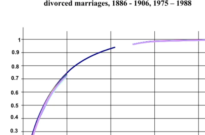
In view of these selection issues, it is reassuring that the cumulative distribution of duration to separation is very stable in time (see Figure 3).23 Individual profiles have
been taken from U.S. Bureau of Census (1909: Table 11) and from annual reports of vital statistics, published by the National Center for Health Statistics (1979 – 1982, 1984 – 1991, 1996). The general shape corresponds to that of an exponential distribution where for t≥ 0. It is steepest in the early years of marriage which is in agreement with the claims of numerous researchers that the risk of separation is highest in the first years of marriage and that it monotonically declines in duration of marriage (Monahan 1962; Plateris 1973). Using data on couples divorced in 1977, Plateris (1981:7–10, Figure 5) notes that separations occurred modally in the first year and that the distribution of all divorces by duration to separation is a decreasing function. This pattern holds in 11 of the 15 states he lists (Plateris 1981:Table 5). It appears in the charity data collected by Marquis (1916), too, and it also holds across states in data from U.S. Bureau of Census (1909:Table 11).
rt
e r t
F(, )=1− −
Overall, about 14% of all marriages that eventually end in divorce separate in the first year of marriage and about three quarters of all such disruptions occur in the first eleven years of marriage. Since the pattern is very stable across the 20th century, it is
plausible that the problem of self-selection is not very severe: the duration profile of
marriage-to-separation is the same among divorced couples in the 1970s and 1980s (when presumably a high proportion of all disrupted marriages ended in divorce) as it was in 1887 – 1906 (when divorce was relatively more expensive and so a smaller proportion of failed marriages could be expected to make it to the court).
Figure 3: Cumulative distribution of duration-to-separation of eventually divorced marriages, 1886 - 1906, 1975 – 1988
1
1886-1906
0.9 1975
1976 0.8
1977
0.7 1978
1979 0.6
1980
0.5 1981
1982 0.4
1983 1984 0.3
1985
0.2 1986
1987 0.1
1988 0
10
0 20 30 40 50
Years of marriage
Source: National Center for Health Statistics (1979-1982, 1984-1991, 1996), U.S. Bureau of the Census (1909)
I adopt the exponential distribution as a basis for the duration profile. Its sole parameter, r, is estimated simply by finding the best fit to the fifteen duration profiles presented in Figure 3. This produces fifteen estimates of r ranging from 0.1305 to 0.1346, all with standard errors below 0.0023. I choose r = 0.133 which would comfortably fall within the 95% confidence interval around any of the fifteen estimates. The duration profile therefore takes the form F(t)=1−e−0.133t.
spouses (large gap tends to destabilize marriage), the order of marriage (second and higher-order marriages are less stable than first marriages), income and living standards of a couple (risk of marital disruption weakly decreases with income), existence of children prior to marriage (increases the risk of disruption). Moreover, it is based on cross-sectional data, yet it is applied to each cohort throughout their lifetime. However, considering the relative scarcity of comprehensive data on marriage disruptions in the past, the adopted methodology is perhaps the closest one can get to actually estimating the rate at which historical marriages disrupted.
4.5 Assumptions – A Summary
Given the lengthy discussion of all the pitfalls in the data, it may be useful, before presenting the results, to summarize the underlying assumptions and to acknowledge their effects on the estimation:
1. In the census, intact marriages are those where both spouses are reported as present in the household. Relaxing this assumption by including individuals who report themselves married but have no spouse living with them would increase the overall total of intact marriages, thereby reducing the estimated proportion ever disrupted, π. It would also introduce a discrepancy between the total married men and total married women.
2. Common-law marriages are absent in the data on marriages solemnized (i.e. on size of individual marriage cohorts) but may be present in the census counts of intact marriages. This assumption acts to inflate the estimated proportion intact (compared to what it properly should be), thereby producing a conservative estimate of proportion ever disrupted, π.
3. The correlation between spouses’ mortalities is ρ = 0.2. Higher values of ρ would decrease incidence of widowhood, thereby increasing the estimated π, especially for the oldest marriage cohorts – and vice versa.
5. The duration profile of marriage-to separation is constant across the period 1860 – 1948. Relaxing this assumption would mostly affect the youngest, most recent marriage cohorts in each census. A steeper profile would produce lower estimates of π while a flatter duration profile would lead to a higher estimated π.
5. Results and sensitivity
πˆ
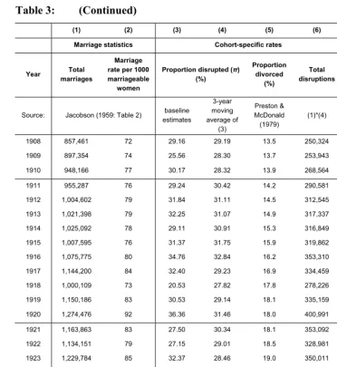
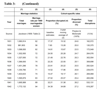
The estimated proportion of each cohort ending in marital disruption, , is presented in Table 3, in columns (3) and (4), and in Figure 4 (baseline estimate). Given that the estimation inevitably contains some error, a three-year centered moving average is also shown to highlight the underlying trend. Period-specific rates of disruption are in column (8) of Table 3 and also in Figure 5. The proportion disrupted declined after the Civil War and then slowly increased for marriage cohorts who wed between 1870 and 1900, staying between 10% and 18%. The upward trend sharply accelerated after the turn of the century and the cohort percentage of disrupted marriages reached a new plateau at about 30% throughout the 1910s and early 1920s. Then it gradually declined and plunged to close to all-time lows for the Great Depression marriage cohorts. In the early 1940s, we can see that World War II marriages witnessed growing disruption with the rate climbing to record levels in the late 1940s.
The proportion of marriages ever disrupted was clearly much more volatile than the proportion ever divorced, as calculated by Preston and McDonald (1979). From the late 1860s,πˆ
increased only slowly and stayed relatively close to the proportion ever divorced. After 1889, however, there is a mild increase in the gradient which becomes steeper after the turn of the century. Between 1906 and 1930 the proportion ever disrupted consistently stayed above 25% (with the exception of the 1918 marriage cohort24) and, even more importantly, well above the cohort divorce rate so that in some
marriage cohorts (1906, for example) fully one half of all marital disruptions never came to any legal closure. This arc of high cohort disruption rates from 1900 to 1930 is a very robust result of the estimation. So, too, is the plunge we can observe during the Great Depression. Another decline in 1938 again corresponds to an economic downturn. Cohort propensity to marriage disruption was clearly closely linked to the economic conditions at the time of marriage.
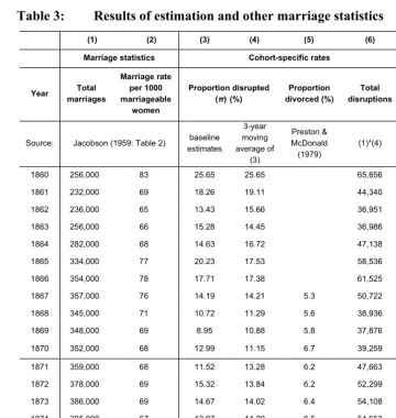
Table 3: Results of estimation and other marriage statistics
(1) (2) (3) (4) (5) (6) (7) (8)
Marriage statistics Cohort-specific rates Period-specific rates
Year Total marriages Marriage rate per 1000 marriageable women Proportion disrupted (π)(%) Proportion divorced (%) Total disruptions Divorce rate Disruption rate
Source: Jacobson (1959: Table 2) baseline estimates 3-year moving average of (3) Preston & McDonald (1979) (1)*(4) Jacobson (1959: Table 42) estimate
1860 256,000 83 25.65 25.65 65,656 1.2
1861 232,000 69 18.26 19.11 44,340 1.1
1862 236,000 65 13.43 15.66 36,951 1.0
1863 256,000 66 15.28 14.45 36,986 1.1
1864 282,000 68 14.63 16.72 47,138 1.4
1865 334,000 77 20.23 17.53 58,536 1.6 7.62
1866 354,000 78 17.71 17.38 61,525 1.8 8.19
1867 357,000 76 14.19 14.21 5.3 50,722 1.5 8.05
1868 345,000 71 10.72 11.29 5.6 38,936 1.5 7.39
1869 348,000 69 8.95 10.88 5.8 37,876 1.6 6.79
1870 352,000 68 12.99 11.15 6.7 39,259 1.5 6.72
1871 359,000 68 11.52 13.28 6.2 47,663 1.6 6.19
1872 378,000 69 15.32 13.84 6.2 52,299 1.7 6.52
1873 386,000 69 14.67 14.02 6.4 54,108 1.7 6.67
1874 385,000 67 12.07 14.20 6.5 54,653 1.8 6.25
1875 409,000 70 15.85 14.34 6.4 58,652 1.8 6.53
1876 405,000 68 15.10 14.80 6.9 59,956 1.8 6.61
1877 411,000 67 13.46 13.81 6.4 56,751 1.9 6.40
1878 423,000 68 12.86 12.33 7.2 52,147 1.9 6.41
1879 438,000 69 10.66 11.88 7.5 52,051 2.0 6.15
Table 3: (Continued)
(1) (2) (3) (4) (5) (6) (7) (8) Marriage statistics Cohort-specific rates Period-specific rates
Year Total marriages
Marriage rate per 1000 marriageable women
Proportion disrupted (π) (%) Proportion divorced (%) Total disruptions Divorce rate Disruption rate
Source: Jacobson (1959: Table 2) baseline estimates 3-year moving average of (3) Preston & McDonald (1979) (1)*(4) Jacobson (1959: Table 42) estimate
1881 464,000 70 10.33 12.60 7.8 58,444 2.3 5.81
1882 484,000 70 15.33 14.31 7.9 69,263 2.4 6.08
1883 501,000 70 17.27 15.42 7.8 77,247 2.4 6.41
1884 485,000 66 13.65 15.30 8.2 74,200 2.4 6.21
1885 507,000 67 14.97 15.42 8.3 78,195 2.3 6.48
1886 534,000 69 17.64 14.12 8.2 75,381 2.5 6.49
1887 513,000 64 9.73 12.83 9.2 65,806 2.7 6.28
1888 535,000 65 11.10 11.08 9.3 59,293 2.7 6.15
1889 563,000 67 12.41 12.03 9.3 67,707 2.9 6.06
1890 570,000 67 12.56 13.13 9.8 74,819 3.0 5.97
1891 592,000 67 14.40 14.46 9.6 85,590 3.1 6.08
1892 601,000 67 16.41 15.20 9.5 91,356 3.1 6.26
1893 601,000 66 14.79 14.38 10.2 86,410 3.1 6.27
1894 588,000 63 11.93 14.22 10.4 83,610 3.0 6.08
1895 620,000 65 15.93 15.29 10.9 94,803 3.2 6.13
1896 635,000 65 18.01 16.20 11.1 102,883 3.3 6.46
1897 643,000 65 14.67 15.29 11.3 98,318 3.4 6.39
1898 647,000 64 13.20 13.54 11.8 87,606 3.6 6.35
1899 673,000 66 12.76 13.53 11.7 91,080 3.7 6.30
1900 709,000 68 14.65 13.88 12.0 98,412 4.0 6.20
1901 742,000 70 14.24 15.50 11.8 114,979 4.2 6.36
1902 776,000 72 17.60 17.29 11.7 134,170 4.2 6.68
1903 818,000 74 20.03 16.89 11.5 138,137 4.3 7.22
1904 815,000 73 13.03 15.83 11.8 129,011 4.3 7.00
1905 842,000 74 14.43 17.89 12.2 150,633 4.3 7.00
1906 895,000 77 26.21 24.50 12.1 219,270 4.4 7.84
Table 3: (Continued)
(1) (2) (3) (4) (5) (6) (7) (8) Marriage statistics Cohort-specific rates Period-specific rates
Year Total marriages
Marriage rate per 1000 marriageable women
Proportion disrupted (π) (%) Proportion divorced (%) Total disruptions Divorce rate Disruption rate
Source: Jacobson (1959: Table 2) baseline estimates 3-year moving average of (3) Preston & McDonald (1979) (1)*(4) Jacobson (1959: Table 42) estimate
1908 857,461 72 29.16 29.19 13.5 250,324 4.4 9.43
1909 897,354 74 25.56 28.30 13.7 253,943 4.5 9.70
1910 948,166 77 30.17 28.32 13.9 268,564 4.5 10.41
1911 955,287 76 29.24 30.42 14.2 290,581 4.8 10.64
1912 1,004,602 79 31.84 31.11 14.5 312,545 4.9 11.42
1913 1,021,398 79 32.25 31.07 14.9 317,337 4.7 11.81
1914 1,025,092 78 29.11 30.91 15.3 316,849 5.0 12.17
1915 1,007,595 76 31.37 31.75 15.9 319,862 5.1 12.26
1916 1,075,775 80 34.76 32.84 16.2 353,310 5.5 12.86
1917 1,144,200 84 32.40 29.23 16.9 334,459 5.7 13.36
1918 1,000,109 73 20.53 27.82 17.8 278,226 5.4 12.57
1919 1,150,186 83 30.53 29.14 18.1 335,159 6.5 12.95
1920 1,274,476 92 36.36 31.46 18.0 400,991 7.7 13.88
1921 1,163,863 83 27.50 30.34 18.1 353,092 7.1 14.06
1922 1,134,151 79 27.15 29.01 18.5 328,981 6.6 13.87
1923 1,229,784 85 32.37 28.46 19.0 350,011 7.2 14.09
1924 1,184,574 80 25.87 28.70 19.4 339,943 7.2 13.81
1925 1,188,334 79 27.86 26.85 19.5 319,097 7.3 13.42
1926 1,202,574 78 26.83 27.19 20.1 326,954 7.4 13.29
1927 1,201,053 77 26.87 26.61 21.0 319,624 7.7 13.10
1928 1,182,497 74 26.13 26.68 21.8 315,436 7.8 12.79
1929 1,232,559 76 27.02 24.70 23.5 304,456 7.9 12.78
Table 3: (Continued)
(1) (2) (3) (4) (5) (6) (7) (8) Marriage statistics Cohort-specific rates Period-specific rates
Year Total marriages
Marriage rate per 1000 marriageable women
Proportion disrupted (π) (%)
Proportion divorced
(%)
Total disruptions
Divorce rate
Disruption rate
Source: Jacobson (1959: Table 2) baseline estimates
3-year moving average of
(3)
Preston & McDonald (1979)
(1)*(4)
Jacobson (1959: Table 42)
estimate
1931 1,060,914 62 17.37 15.32 24.6 162,572 7.0 11.39
1932 981,903 56 7.65 13.28 25.0 130,375 6.1 10.20
1933 1,098,000 62 14.81 15.67 23.5 172,049 6.1 9.68
1934 1,302,000 72 24.55 20.28 24.7 264,076 7.4 9.95
1935 1,327,000 72 21.49 22.76 25.3 302,054 7.8 9.88
1936 1,369,000 74 22.25 22.55 25.1 308,698 8.3 9.93
1937 1,451,296 78 23.91 20.22 25.5 293,524 8.6 10.12
1938 1,330,780 71 14.52 17.96 25.8 239,070 8.3 9.57
1939 1,403,633 74 15.47 19.17 26.1 269,069 8.4 9.20
1940 1,595,879 83 27.52 25.07 25.4 400,056 8.7 9.83
1941 1,695,999 89 32.21 31.38 26.2 532,131 9.4 10.77
1942 1,772,132 94 34.39 34.89 27.2 618,287 10.0 11.66
1943 1,577,050 84 38.06 35.87 27.5 565,629 10.9 12.40
1944 1,452,394 76 35.14 31.00 27.7 450,282 12.3 12.58
1945 1,612,992 84 19.80 37.98 25.1 612,637 14.3 12.02
1946 2,291,045 120 59.00 36.74 24.3 841,779 18.2 15.53
1947 1,991,878 107 31.43 46.64 25.7 929,007 13.9 15.81
1948 1,811,155 98 49.49 26.4 11.6 16.69
Figure 4: Cohort rates of marital disruption
0 10 20 30 40 50 60
1860 1870 1880 1890 1900 1910 1920 1930 1940
Proportion ever disrupted - baseline estimate
3-year moving average of baseline estimate
Proportion ever divorced (Preston & McDonald, 1979)
Note: For specific numerical values, see Table 3.
Using the disruption profile, specified in section 4.4, I converted the cohort rates into period rates of disruption (Figure 5). In its basic outlines, this graph is similar to the cohort rates because a majority of disruptions occur in the first five years of marriage. The period disruption rate also grew vigorously in the first two decades of the 20th century, excepting a dip during the epidemic of 1918 – 1919. After a peak in 1923,
there was a gradual decline which turned into a dive with the onset of the Great Depression.25
The precision of these marital disruption rates depends on the precision of inputs. They are most sensitive to variation in mortality rates, somewhat sensitive to variation
in the proportion intact and least sensitive to variation in duration profile. However, the underlying movements in disruption rates are not affected by any of these variations.
Figure 5: Legal vs. Real ends of marriage, period rates per 1000 marriages
0.0 2.0 4.0 6.0 8.0 10.0 12.0 14.0 16.0 18.0 20.0
1860 1870 1880 1890 1900 1910 1920 1930 1940
Divorce rate (Jacobson, 1959)
Disruption rate - baseline estimate
Note: For specific values, see Table 3.
The sensitivity to the proportion of intact marriages is apparent from Figure 6. The late 19th century marriage cohorts can be observed both in the 1900 census and in the
Figure 6: Various estimates of proportion ever disrupted
0.00 0.05 0.10 0.15 0.20 0.25 0.30 0.35 0.40 0.45 0.50
1860 1865 1870 1875 1880 1885 1890 1895 1900 1905
based on 1900 census
based on 1910 census
Note: See section 5.
absorbed close to a half of what in other censuses would be “married, spouse absent” respondents.
Figure 7: Various estimates of proportion ever disrupted
-0.05 0.00 0.05 0.10 0.15 0.20 0.25 0.30 0.35 0.40 0.45 0.50
1860 1865 1870 1875 1880 1885 1890 1895 1900 1905
1900 census - married, spouse present 1910 census - married, spouse present 1900 census - married
1910 census - married
Note: See section 5.
Table 4: Estimates of π (in %) and variation in parameters
Mortality r
Benchmark estimate
10% -10% 0.120 0.147
1907 32.86 25.73 39.21 32.44 33.25
1908 29.16 23.12 34.74 28.91 29.41
1909 25.56 18.76 31.73 25.30 25.81
1910 30.17 24.51 35.41 29.91 30.43
1911 29.24 24.05 34.08 29.02 29.45
1912 31.84 27.12 36.30 31.64 32.07
1913 32.25 27.75 36.48 32.06 32.46
1914 29.11 23.85 33.90 28.82 29.40
1915 31.37 27.35 35.17 31.25 31.52
1916 34.76 30.96 38.34 34.64 34.92
1917 32.40 28.53 36.05 32.30 32.54
1918 20.53 15.91 24.78 20.44 20.65
1919 30.53 27.08 33.80 30.52 30.59
1920 36.36 33.42 39.15 36.40 36.40
1921 27.50 23.88 30.83 27.46 27.59
1922 27.15 24.24 29.93 27.25 27.12
1923 32.37 30.03 34.64 32.57 32.26
1924 25.87 23.07 28.52 26.02 25.78
1925 27.86 25.62 30.02 28.11 27.70
1926 26.83 24.47 29.09 27.10 26.66
1927 26.87 24.84 28.83 27.21 26.64
1928 26.13 24.29 27.92 26.52 25.85
1929 27.02 24.84 29.08 27.42 26.74
1930 20.95 18.86 22.93 21.32 20.67
1931 17.37 15.75 18.92 17.73 17.09
1932 7.65 5.74 9.45 7.82 7.52
1933 14.81 13.41 16.17 15.20 14.50
1934 24.55 23.15 25.88 25.26 23.97
1935 21.49 20.16 22.75 22.18 20.93
1936 22.25 21.04 23.39 23.04 21.60
1937 23.91 22.72 25.03 24.83 23.14
Table 4: (Continued)
Mortality r
Benchmark estimate
10% -10% 0.120 0.147
1939 15.47 14.45 16.44 16.19 14.86
1940 27.52 26.83 28.20 28.92 26.33
1941 32.21 31.21 33.07 33.96 30.71
1942 34.39 33.74 35.03 36.44 32.63
1943 38.06 37.48 38.64 40.52 35.94
1944 35.14 34.57 35.71 37.59 33.02
1945 19.80 19.30 20.30 21.28 18.51
1946 59.00 58.56 59.43 63.75 54.84
1947 31.43 31.01 31.84 34.14 29.05
1948 49.49 49.13 49.85 54.10 45.47
A similar +/-10% variation in the parameter r which governs the duration profile of marital disruption has the opposite effect: it most strongly affects the most recent cohorts. These cohorts had only been married for a short time as of the date of the census and any inference about their lifetime rate of marital disruption is open to relatively larger error than it is in case of cohorts that have most of their disruptions behind them. Even so, the range is the greatest for the marriage cohort of 1946 where the estimated disruption rate varies by +/-4 percentage point.
One of the assumptions touched on the problem of common-law marriages. For reasons explained above, it has been assumed that these marriages, which are absent from Jacobson’s (1959) tallies because they did not go through a formal solemnization, were too few to affect the estimated values. However, it is illuminating to see how the estimates would be affected if the assumption were different.
1948. Again, not surprisingly, such estimates are about six percentage points higher than the benchmark in 1860 and then they gradually converge as the assumed incidence of common-law marriage declines. The conclusion from this exercise is that the incidence of common-law marriage acts as a shifter of the estimates but that it does not affect the main trends in the estimated disruption rate. Moreover, as could be expected, the effect is relatively small, given that the assumed incidence of common-law marriage is small.26 Finally, whatever incidence is assumed, the resulting estimates turn out to be
higher than the benchmark values. In other words, the benchmark can be viewed as a conservative estimate.
Figure 8: Estimated disruption rate under various assumptions about incidence of common-law marriage
0.00 0.05 0.10 0.15 0.20 0.25 0.30 0.35 0.40 0.45 0.50
1860 1865 1870 1875 1880 1885 1890 1895 1900 1905 1910 1915 1920 1925 1930 1935 1940 1945 (A) benchmark (3-year MA - Table 3, col. (4))
(B) assuming 5% incidence of common-law marriage (3-year MA)
(C) assuming geometrically falling incidence of common-law marriage (3-year MA)
Note: See section 5.
6. Further conceptual issues
It is much harder to establish the reality of a marital disruption than it is of a divorce. The census is only a snapshot of the population, taken every decade. It therefore provides insufficient or inaccurate information about many aspects of the population’s evolution between census years. With respect to marital disruption, this presents a particular problem in those cases where a separated couple may reunite after some – potentially even relatively extensive – period of time. Since, legally, such movement would not change the marital status of the couple, who would be observed in a census year as an intact marriage, there is no way to know how many and how long such intermittent disruptions were. As a result, the disruption statistic could seriously underestimate the incidence of marital disruptions.
Intermittent disruption is, of course, still a disruption in the same way that a divorced couple can remarry each other a few years later and their divorce still rightfully appears in the divorce statistics. However, the nature of the marital situation in cases of repeated short-term desertions need not be as clear-cut as it is with divorces which become a statistic at the strike of the gavel. Families, where the husband leaves regularly at the time of his pregnant wife’s confinement and comes back shortly thereafter (Smith, 1901:4), though obviously dysfunctional, are clearly not failures in the same way as those where a husband is gone for, say, five years and counting. Eubank (1916:41–45) argues that these “intermittent husbands” – the chronic, repeat deserters – in fact, do not wish to end their marriage: rather, they use it as a spring-board for occasional (sometimes regular, periodic and even seasonal) but relatively short-term absences. Such marriages could probably be regarded as still intact, if dysfunctional, and it is likely that such intermittent husbands would be recorded in the census as living with the family. On the other hand, in those cases, where the separation has been long term – such as over a year – a firmer inference can be made that both spouses have probably come to regard the marriage as de facto terminated.
The second issue is that period from 1930 to 1940 presents a seeming paradox: in those cohorts, there seem to be fewer lifetime disruptions than there were lifetime divorces. This is conceptually impossible, given that divorces are a subset of disruptions. The two series were calculated from different sources and using different techniques. Preston and McDonald (1979) obtained their estimates from the available evidence on divorces. American divorce statistics were consistently collected for period 1867-1906, the year 1916, the ten-year period from 1922 to 1932 and then again from 1949 until 1988. These government reports included duration data of varying degrees of precision.27 Between the years covered by the government reports, estimates of total
divorces granted in the United States are available from Jacobson (1959: Table 42) or Plateris (1973: Table 1) but not their distribution by duration. So, for the period 1933 – 1948, Preston and McDonald (1979) employed “linear interpolation between distributions of divorce by duration in 1927 – 31 and 1949 – 1953” (Preston and McDonald 1979:24). The period 1933 – 1948 happens to be the most volatile time in American marital relations. Figure 5 illustrates that the divorce rate went from 6.1 in 1933 to 18.2 in 1947, before falling back to 11.6 in 1948. Marriage rate climbed from 56 marriages per 1000 marriageable women in 1932 to 120 in 1946 and then fell to 98 by 1948. These wild gyrations in marriage and divorce rates indicate that estimates based on interpolation are likely to miss significant amount of variation and put too much emphasis on the underlying trends. Moreover, Jacobson’s (1949:Figure 6) estimates of divorce rate by duration of marriage show that the Great Depression acted to reduce the divorce rate of relatively new marriages while leaving divorce rates of older marriages mostly constant. The reverse was true after the end of World War Two: divorce rates among young marriages spiked, while older marriages were mostly unaffected.
When all these factors are combined, they likely introduced considerable variability to the duration distribution of divorces between 1933 and 1948: few marriages were celebrated during the Great Depression and those that proved unhappy were strongly discouraged from a divorce by the hard times, whereas struggling marriages from the 1920s were not as strongly discouraged. On the other hand, the late 1930s/early 1940s marriage cohorts were relatively large and they were much more divorce-happy in 1946 – 1948 than the marriages from the 1930s. In fact, even if the Great Depression marriages were as prone to divorce as the 1940s marriages, they would have contributed relatively little to overall divorces because these cohorts were 50% smaller than the 1940s marriage cohorts. For all these reasons the estimates of Preston and McDonald (1979) may understate the wild fluctuations of the Great Depression and the Second World War times and that could be why their cohort rates of divorce are higher than the present estimates of cohort rates of disruption.
Like the cohort measures of marriage failure, the period measures were also closely tied with the economy, as is clear from Figure 5 and columns (7) and (8) of Table 3. The economic stagnation of most of the 1880s coincides with stagnation in disruption rate. After 1900, one can see a new upward trend. The disruption rate naturally declines during the Great Depression: disruptions are most prevalent in early years of married life, so the small marriage cohorts of the 1930s produced relatively fewer disruptions and so a low disruption rate. The disruption rate increases throughout the 1940s, with the exception of 1945.
In 1944 – 1946, the divorce rate exceeds the disruption rate but unlike with cohort measure, this is not necessarily a paradox: it merely indicates that marriages which broke down under the strains of the Depression or the War were only officially divorced a few years later. Generally, one can expect some delay between a separation and a divorce: it is therefore plausible to argue that many of the marriages which were disrupted in 1937 – 1944 were then converted into divorces in the immediately post-war years. This would also closely correspond with Jacobson’s (1949) assessment that it was the most recent marriages that experienced a particularly strong spike in divorce rate in 1947.
The third important conceptual issue is that the estimation lacks any explicit specification of period effects. Some period effects, such as the influenza epidemic of 1918-1919, operate through the mortality rates which affect all the marriage cohorts that lived through it and as such are therefore accounted for in the estimation. Non-death-related period effects, however, are not controlled for. This shortcoming is the price paid for relying on the census (which is a snapshot at one point in time) to infer something about the respondents’ course of life: the census presents an outcome shaped by both cohort effects and period effects. But while the cohort effects can be separated (with the aid of variable DURMARR), the period effects cannot. This problem is partly offset by the shape of the duration profile: given that most marriage break-ups occur in the first few years of marriage, one can argue that the period effects exert their greatest influence on the most recent marriages and so in this way the period and cohort effects are basically conflated. To what extent is this offsetting influence a sufficient cure for this issue is unclear.
7. Conclusion
The estimates of marital disruption presented in this paper are the first serious attempt to quantify a grey area of marriage dynamics that occurred under the radar of the law. While marriage and divorce usually are a matter of public record, desertion and separation often went unrecorded. Using available information on mortality and census records on intact marriages, I infer that marriages that have neither ended in widowhood, nor remained intact, must have been disrupted – whether with the aid of the court or without it.
cohort and period rates of disruption diverged from the rates of divorce. A growing proportion of marriages were disrupted without being divorced, leaving the spouses (especially wives) in a legal limbo and under a considerable economic and social strain. Not surprisingly, this period of rapidly increasing disruptions witnessed a proliferation of literature by social scientists, legislators and social workers on the problem of family desertion. It was only in the 1930s and 1940s when the rates of disruption and divorce converged again, first through a decline in the disruption rate (during the Great Depression), then through a concurrent increase of both. This probably reflects the fact that divorce was getting cheaper not only in terms of time and money but also in terms of social prestige lost (as public acceptance of divorce became gradually more widespread).
As one of the oldest and most diverse human institution, marriage was always rich in aspects that stood aside from formal law. The estimated unrecorded marital disruptions provide a glimpse of how prevalent such extra-legal behavior may have been in the United States between 1860 and 1948.